8. Assessing Product Reliability
8.1. Introduction
8.1.6. What are the basic lifetime distribution models used for non-repairable populations?

8.1.6.6.

Fatigue life (Birnbaum-Saunders)

A model based on cycles of stress causing degradation or crack growth

In 1969, Birnbaum and Saunders described a life distribution model that could be derived from a physical fatigue process where crack growth causes failure. Since one of the best ways to choose a life distribution model is to derive it from a physical/statistical argument that is consistent with the failure mechanism, the Birnbaum-Saunders Fatigue Life Distribution is worth considering. 

• Formulas and Plots for the Birnbaum-Saunders Model
• Derivation and Use of the Birnbaum-Saunders Model
• Dataplot Functions for the Birnbaum-Saunders Model

Formulas and Plots for the Birnbaum-Saunders Model

Formulas and shapes for the Fatigue Life model

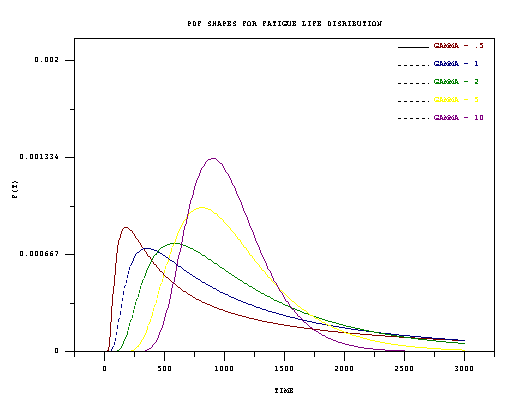
The PDF, CDF, mean and variance for the Birnbaum-Saunders Distribution are shown below. The parameters are:,  a shape parameter; µ, a scale parameter. These are the parameters used in Dataplot, but there are other choices also common in the literature (see the parameters used for the derivation of the model).

PDF shapes for the model vary from highly skewed and long tailed (small gamma values) to nearly symmetric and short tailed as gamma increases. This is shown in the figure below.

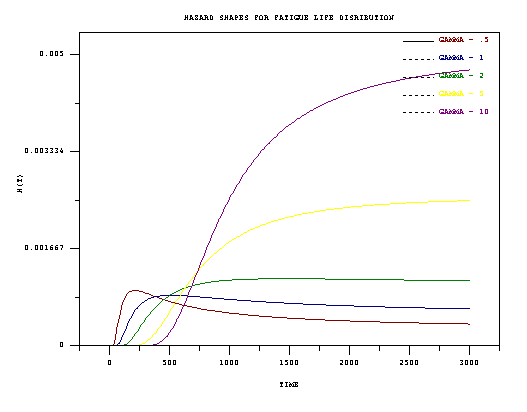
Corresponding failure rate curves are shown in the next figure.

If crack growth in each stress cycle is a random amount independent of past cycles of growth, the Fatigue Life mode model may apply.

Derivation and Use of the Birnbaum-Saunders Model: 

Consider a material that continually undergoes cycles of stress loads. During each cycle, a dominant crack grows towards a critical length that will cause failure. Under repeated application of n cycles of loads, the total extension of the dominant crack can be written as 

and we assume the Y_j are independent and identically distributed non-negative random variables with mean µ and variance . Suppose failure occurs at the N-th cycle, when W_n first exceeds a constant critical value w. If n is large, we can use a central limit theorem argument to conclude that 

Since there are many cycles, each lasting a very short time, we can replace the discrete number of cycles N needed to reach failure by the continuous time t_f needed to reach failure. The cdf F(t) of t_f is given by 

Here  denotes the standard normal cdf. Writing the model with parameters  and  is an alternative way of writing the Birnbaum-Saunders distribution that is often used      (, as compared to the way the formulas were parameterized earlier in this section). 

Note:
The critical assumption in the derivation, from a physical point of view, is that the crack growth during any one cycle is independent of the growth during any other cycle. Also, the growth has approximately the same random distribution, from cycle to cycle. This is a very different situation from the proportional degradation argument used to derive a log normal distribution model, with the rate of degradation at any point in time depending on the total amount of degradation that has occurred up to that time. 

This kind of physical degradation is consistent with Miner's Rule.

The Birnbaum-Saunders assumption, while physically restrictive, is consistent with a deterministic model from materials physics known as Miner's Rule (Miner's Rule implies that the damage that occurs after n cycles, at a stress level that produces a fatigue life of N cycles, is proportional to n/N). So, when the physics of failure suggests Miner's Rule applies, the Birnbaum-Saunders model is a reasonable choice for a life distribution model.

Dataplot commands for the Fatigue Life model

Dataplot Functions for the Birnbaum-Saunders Model

The PDF for a Birnbaum-Saunders (Fatigue Life) distribution with parameters µ,  is evaluated at time t by: 

LET PDF = FLPDF(t, , 0, µ).

The CDF is 

LET CDF = FLCDF(t, , 0, µ).

To generate 100 random numbers, when µ = 5000,  = 2, for example, type the following Dataplot commands: 

LET GAMMA = 2
LET DATA = FATIGUE LIFE RANDOM NUMBERS FOR 
    I = 1 1 100
LET DATA = 5000*DATA

Finally, we can do a Fatigue Life Probability Plot of the 100 data points in DATA by 

LET GAMMA = 2
FATIGUE LIFE PROBABILITY PLOT DATA

and the points on the resulting plot (shown below) line up roughly on a straight line, as expected for data correctly modeled by the Birnbaum-Saunders distribution. 

Notes

1. We set GAMMA equal to 2 before doing the probability plot because we knew its value. If we had real experimental data (with no censoring), first we would run PPCC to estimate gamma. The command is: FATIGUE LIFE PPCC PLOT DATA. To see the estimated value of gamma we would type WRITE SHAPE. Then, we would type LET GAMMA = SHAPE before running the Fatigue Life Probability Plot.
2. The slope of the line through the points on the probability plot is an estimate of the scale parameter µ.