8. Assessing Product Reliability
8.4. Reliability Data Analysis
8.4.2. How do you fit an acceleration model?

8.4.2.2.

Maximum likelihood

The maximum likelihood method can be used to estimate distribution and acceleration model parameters at the same time

The Likelihood equation for a multi-cell acceleration model starts by computing the Likelihood functions for each cell, as was described earlier. Each cell will have unknown life distribution parameters that, in general, are different. For example, if a lognormal model is used, each cell might have its own T₅₀ and .

Under an acceleration assumption, however, all the cells contain samples from populations that have the same value of  (the slope does not change for different stress cells). Also, the T₅₀'s are related to one another by the acceleration model; they all can be written using the acceleration model equation with the proper cell stresses put in. 

To form the Likelihood equation under the acceleration model assumption, simply rewrite each cell Likelihood by replacing each cell T₅₀ by its acceleration model equation equivalent and replacing each cell sigma by the same one overall . Then, multiply all these modified cell Likelihoods together to obtain the overall Likelihood equation. 

Once you have the overall Likelihood equation, the maximum likelihood estimates of sigma and the acceleration model parameters are the values that maximize this Likelihood. In most cases, these values are obtained by setting partial derivatives of the log Likelihood to zero and solving the resulting (non-linear) set of equations. 

The method is complicated and requires specialized software

As you can see, the procedure is complicated and computationally intensive, and only practical if appropriate software is available. It does have many desirable features such as:

• the method can, in theory at least, be used for any distribution model and acceleration model and type of censored data
• estimates have "optimal" statistical properties as sample sizes (i.e., numbers of failures) become large
• approximate confidence bounds can be calculated
• statistical tests of key assumptions can be made using the likelihood ratio test. Some common tests are:
• the life distribution model versus another simpler model with fewer parameters (i.e., a 3-parameter Weibull versus a 2-parameter Weibull, or a 2-parameter Weibull vs an exponential)
• the constant slope from cell to cell requirement of typical acceleration models
• the fit of a particular acceleration model

In general, the recommendations made when comparing methods of estimating life distribution model parameters also apply here. Software incorporating acceleration model analysis capability, while rare just a few years ago, is now readily available and many companies and universities have developed their own proprietary versions. 

Example Comparing Graphical Estimates and MLE 's

Arrhenius example comparing graphical and MLE method results

The data from the 3-stress-cell Arrhenius example given in  the preceding section were analyzed using a proprietary MLE program that could fit individual cells and also do an overall Arrhenius fit. The tables below compare results. 
 
 

	Graphical Estimates		MLE's
	ln T50	Sigma	ln T50	Sigma
Cell 1	8.17	.91	8.89	1.21
Cell 2	6.42	.66	6.47	.71
Cell 3	5.32	.81	5.33	.81

Acceleration Model Overall Estimates

	H	Sigma	ln A
Graphical	.808	.74	-18.312
MLE	.863	.77	-19.91

Note that when there were a lot of failures and little censoring, the two methods were in fairly close agreement. Both methods were also in close agreement on the Arrhenius model results. However, even small differences can be important when projecting reliability numbers at use conditions. In this example, the CDF at 25°C and 100,000 hours projects to .014 using the graphical estimates and only .003 using the MLE estimates.

MLE method tests models and gives confidence intervals

The Maximum Likelihood program also tested whether parallel lines (a single sigma) were reasonable and whether the Arrhenius model was acceptable. The three cells of data passed both of these Likelihood Ratio tests easily. In addition, the MLE program output included confidence intervals for all estimated parameters. 

SAS JMP™ software (previously used to find single cell Weibull MLE's) can also be used for fitting acceleration models. This is shown next. 

Using SAS JMP™Software To Fit Reliability Models

Detailed explanation of how to use JMP software to fit an Arrhenius model

If you have JMP on your computer, set up to run as a browser application, click here to load a lognormal template JMP spreadsheet named arrex.jmp. This template has the Arrhenius example data already entered. The template extends JMP's analysis capabilities beyond the standard JMP routines by making use of JMP's powerful "Nonlinear Fit" option (links to blank templates for both Weibull and lognormal data are provided at the end of this page). 

First, a standard JMP reliability model analysis for these data will be shown. By working with screen windows showing both JMP and the Handbook, you can try out the steps in this analysis as you read them. Most of the screens below are based on JMP 3.2 platforms, but comparable analyses can be run with JMP 4.

The first part of the spreadsheet should appear as illustrated below.

Steps For Fitting The Arrhenius Model Using JMP's "Survival" Options

1. The "Start Time" column has all the fail and censor times and "Censor" and "Freq" were entered as shown previously. In addition, the temperatures in degrees C corresponding to  each row were entered in "Temp in C". That is all that has to be entered on the template; all other columns are calculated as needed. In particular, the "1/kT" column contains the standard Arrhenius 1/kT values for the different temperature cells.

2. To obtain a plot of all three cells, along with individual cell lognormal parameter estimates, choose "Kaplan - Meier" (or "Product Limit") from the "Analysis" menu and fill in the screen as shown below. 

Column names are transferred to the slots on the right by highlighting them and clicking on the tab for the slot. Note that the "Temp in C" column is transferred to the "Grouping" slot in order to analyze and plot each of the three temperature cells separately.

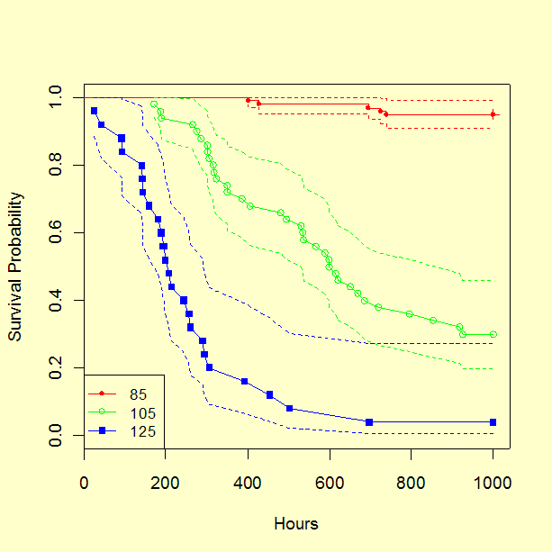
Clicking "OK" brings up the analysis screen below. All plots and estimates are based on individual cell data, without the Arrhenius model assumption. Note: To obtain the lognormal plots, parameter estimates and confidence bounds, it was necessary to click on various "tabs" or "check" marks - this may depend on the software release level.

This screen does not give -LogLikelihood values for the cells. These are obtained from the "Parametric Model" option in the "Survival" menu (after clicking "Analyze").

3. First we will use the "Parametric Model" option to obtain individual cell estimates. On the JMP data spreadsheet (arrex.jmp), select all rows except those corresponding to cell 1 (the 85 degree cell) and choose "Exclude" from the "Row" button options (or do "ctrl+E"). Then click "Analyze" followed by "Survival" and "Parametric Model". Enter the appropriate columns, as shown below. Make sure you use "Get Model" to select "lognormal" and  click "Run Model".

This will generate a model fit screen for cell 1. Repeat for cells 2 and 3. The three resulting model fit screens are shown below.

Note that the model estimates and bounds are the same as obtained in step 2, but these screens also give -LogLikelihood values. Unfortunately, as previously noted, these values are off by the sum of the {ln(times of failure)} for each cell. These sums for the three cells are 31.7871, 213.3097 and 371.2155, respectively. So the correct cell -LogLikelihood values for comparing with other MLE programs are 53.3546, 265.2323 and 156.5250, respectively. Adding them together yields a total -LogLikelihood of 475.1119 for all the data fit with separate lognormal parameters for each cell (no Arrhenius model assumption). 

4. To fit the Arrhenius model across the three cells go back to the survival model screen, this time with all the data rows included and the "1/kT" column selected and put into the "Effects in Model" box via the "Add" button. This adds the Arrhenius temperature effect to the MLE analysis of all the cell data. The screen looks like:

Clicking "Run Model" produces

The MLE estimates agree with those shown in the tables earlier on this page. The -LogLikelihood for the model is given under "Full" in the output screen (and should be adjusted by adding the sum of all the ln failure times from all three cells if comparisons to other programs might be made). This yields a model -LogLikelihood of  105.4934 + 371.2155 = 476.7089. 

5. The likelihood ratio test statistic for the Arrhenius model fit (which also incorporates the single sigma acceleration assumption) is - 2Log, with denoting the difference between the LogLikelihoods with and without the Arrhenius model assumption. Using the results from steps 3 and 4, we have - 2Log = 2 × (476.709 - 475.112) = 3.194. The degrees of freedom (dof) for the Chi-Square test statistic is 6 - 3 = 3, since six parameters were reduced to three under the acceleration model assumption. The chance of obtaining a value 3.194 or higher is 36.3% for a Chi Square distribution with 3 dof, which indicates an acceptable model (no significant lack of fit).

This completes a JMP 3.2 Arrhenius model analysis of the three cells of data. Since the Survival Modeling screen allows any "effects" to be included in the model, if different cells of data had different voltages, the "ln V" column could be added as an effect to fit the Inverse Power Law voltage model. In fact, several effects can be included at once if more than one stress varies across cells. Cross product stress terms could also be included by adding these columns to the spreadsheet and adding them in the model as additional "effects". 

Arrhenius example using special JMP template and "Nonlinear Fit"

Steps For Fitting The Arrhenius Model Using the "Nonlinear Fit" Option and Special JMP Templates

There is another powerful and flexible tool included within JMP that can use MLE methods to fit reliability models. While this approach requires some simple programming of JMP calculator equations, it offers the advantage of extending JMP's analysis capabilities to readout data (or truncated data, or any combination of different types of data). Templates (available below) have been set up to cover lognormal and Weibull data. The spreadsheet used above (arrex.jmp) is just a partial version of the lognormal template, with the Arrhenius data entered. The full templates can also be used to project CDF's at user stress conditions, with confidence bounds.

The following steps work with arrex.jmp because the "loss" columns have been set up to calculate -LogLikelihoods for each row. 

1. Load the arrex.jmp spreadsheet and Click "Analyze" on the Tool Bar and choose "Nonlinear Fit".

2. Select the Loss (w/Temp) column and click "Loss" to put "Loss (w/Temp)" in the box. This column on the spreadsheet automatically calculates the - LogLikelihood values at each data point for the Arrhenius/lognormal model. Click "OK" to run the Nonlinear Analysis.

3. You will next see a "Nonlinear Fit" screen. Select "Loss is -LogLikelihood" and click the "Reset" and "Go" buttons to make sure you have a new analysis. The parameter values for the constant ln A (labeled "Con"), DH and sig will appear and the value of - LogLikelihood is given under the heading "SSE". These numbers are -19.91, 0.863, 0.77 and 476.709, respectively. You can now click on "Confid Limits" to obtain upper and lower confidence limits for these parameters. The stated value of "Alpha = .05" means that the interval between the limits is a  95% confidence interval. At this point your "Nonlinear Fit" screen appears as follows

:

4. Next you can run each cell separately by excluding all data rows corresponding to other cells and repeating steps 1 through 3. For this analysis, select the "Loss (w/o Stress)" column to put in "Loss" in step 2, since a single cell fit does not use temperature . The numbers should match the table shown earlier on this page. The three cell -LogLikelihood values are 53.355, 265.232 and 156.525. These add to 475.112, which is the minimum -loglikelihood possible, since it uses 2 independent parameters to fit each cell separately (for a total of six parameters, overall).

The likelihood ratio test statistic for the Arrhenius model fit (which also incorporates the single sigma acceleration assumption) is - 2Log l = 2 x (476.709 - 475.112) = 3.194. Degrees of freedom for the Chi-Square test statistic is 6 - 3 = 3, since six parameters were reduced to three under the acceleration model assumption. The chance of obtaining a value of 3.194 or higher is 36.3% for a Chi-Square distribution with 3 dof, which indicates an acceptable model (no significant lack of fit).

For further examples of JMP reliability analysis there is an excellent collection of JMP statistical tutorials put together by Professor Ramon Leon and one of his students, Barry Eggleston, available on the Web at http://www.nist.gov/cgi-bin/exit_nist.cgi?url=http://web.utk.edu/~leon/jmp/.

Data entry on JMP templates for general reliability data

How To Use JMP Templates For Lognormal or Weibull Data (Including Acceleration Model Analysis)

With JMP installed to run as a browser application, you can click on weibtmp.jmp or lognmtmp.jmp and load (and save for later use) blank templates similar to the one shown above, for either Weibull or lognormal data analysis. Here's how to enter any kind of data on either of the templates.

Typical Data Entry

1. Any kind of censored or truncated or readout data can be entered. The rules are as follows for the common case of (right) censored reliability data:
 

i) Enter exact failure times in the "Start Time" column, with "0" in the "Cens" column and the number of failures at that exact time in the "Freq" column.

ii) Enter temperature in degrees Celsius for the row entry in "Temp in C", whenever data from several different operating temperatures are present and an Arrhenius model fit is desired.

iii) Enter voltages in "Volt" for each row entry whenever data from several different voltages are present and an Inverse Power Law model fit is desired. If both temperatures and voltages are entered for all data rows, a combined two-stress model can be fit.

iv) Put censor times (when unfailed units are removed from test, or no longer observed)  in the "Start Time" column, and enter "1" in the "Cens" column. Put the number of censored units in the "Freq" column.

v) If readout (also known as interval) data are present, put the interval start time and stop time in the corresponding columns and "2" in the "Cens" column. Put the number of failures during the interval in the "Freq" column. If the number of failures is zero, it doesn't matter if you include the interval, or not. 

Using The Templates For Model Fitting and CDF Projections With Bounds

Pick the appropriate template; weibtmp.jmp for a Weibull fit, or lognmtmp.jmp for a lognormal fit. Follow this link for documentation on the use of these templates. Refer to the Arrhenius model example above for an illustration of how to use the JMP non-linear fit platform with these templates.

A few tricks are needed to handle the rare cases of truncated data or left-censored data. These are described in the template documentation and also repeated below (since they work for the JMP survival platform and can be used with other similar kinds of reliability analysis software .

How to handle truncated or left-censored data using JMP templates

JMP Template Data Entry For Truncated or Left-Censored Weibull or Lognormal Data

Left censored data means all exact times of failure below a lower cut-off time T₀ are unknown, but the number of these failures is known. Merely enter an interval with start time 0 and stop time T₀ on the appropriate template and put "2" in the "Cens" column and the number in the "Freq" column.

Left truncated data means all data points below a lower cut off point T₀ are unknown, and even the number of such points is unknown. This situation occurs commonly for measurement data, when the measuring instrument has a lower threshold detection limit at T₀. Assume there are n data points (all above T₀) actually observed. Enter the n points as you normally would on the appropriate template ("Cens" gets 0 and "Freq" gets 1) and add a start time of T₀ with a "Cens" value of 1 and a "Freq" value of -n (yes, minus n!). 

Right truncated data means all data points above an upper cut-off point T₁ are unknown, and even the number of such points is unknown. Assume there are n data points (all below T₁) actually observed. Enter the n points as you normally would on the appropriate template ("Cens" gets 0 and "Freq" gets 1) and add a start time of  0 and a stop time of T₁ with a "Cens" value of 2 and a "Freq" value of -n (yes, minus n!)