1.3.3.32. 4-Plot

1. Exploratory Data Analysis 1.3. EDA Techniques 1.3.3. Graphical Techniques: Alphabetic 1.3.3.32. 4-Plot
Purpose: Check Underlying Statistical Assumptions	The 4-plot is a collection of 4 specific EDA graphical techniques whose purpose is to test the assumptions that underlie most measurement processes. A 4-plot consists of a run sequence plot; lag plot; histogram; normal probability plot. If the 4 underlying assumptions of a typical measurement process hold, then the above 4 plots will have a characteristic appearance (see the normal random numbers case study below); if any of the underlying assumptions fail to hold, then it will be revealed by an anomalous appearance in one or more of the plots. Several commonly encountered situations are demonstrated in the case studies below. Although the 4-plot has an obvious use for univariate and time series data, its usefulness extends far beyond that. Many statistical models of the form \[ Y_{i} = f(X_{1}, ... 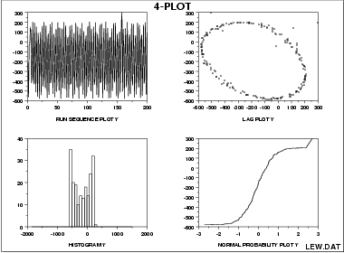, X_{k}) + E_{i} \] have the same underlying assumptions for the error term. That is, no matter how complicated the functional fit, the assumptions on the underlying error term are still the same. The 4-plot can and should be routinely applied to the residuals when fitting models regardless of whether the model is simple or complicated.
Sample Plot: Process Has Fixed Location, Fixed Variation, Non-Random (Oscillatory), Non-Normal U-Shaped Distribution, and Has 3 Outliers.	This 4-plot of the LEW.DAT data set reveals the following: the fixed location assumption is justified as shown by the run sequence plot in the upper left corner. the fixed variation assumption is justified as shown by the run sequence plot in the upper left corner. the randomness assumption is violated as shown by the non-random (oscillatory) lag plot in the upper right corner. the assumption of a common, normal distribution is violated as shown by the histogram in the lower left corner and the normal probability plot in the lower right corner. The distribution is non-normal and is a U-shaped distribution. there are several outliers apparent in the lag plot in the upper right corner.
Definition: 1. Run Sequence Plot; 2. Lag Plot; 3. Histogram; 4. Normal Probability Plot	The 4-plot consists of the following: Run sequence plot to test fixed location and variation. Vertically: Y_i Horizontally: i Lag Plot to test randomness. Vertically: Y_i Horizontally: Y_i-1 Histogram to test (normal) distribution. Vertically: Counts Horizontally: Y Normal probability plot to test normal distribution. Vertically: Ordered Y_i Horizontally: Theoretical values from a normal N(0,1) distribution for ordered Y_i
Questions	4-plots can provide answers to many questions: Is the process in-control, stable, and predictable? Is the process drifting with respect to location? Is the process drifting with respect to variation? Are the data random? Is an observation related to an adjacent observation? If the data are a time series, is white noise? If the data are a time series and not white noise, is it sinusoidal, autoregressive, etc.? If the data are non-random, what is a better model? Does the process follow a normal distribution? If non-normal, what distribution does the process follow? Is the model \[ Y_{i} = A_0 + E_{i} \] valid and sufficient? If the default model is insufficient, what is a better model? Is the formula \[ s_{\bar{Y}} = s/\sqrt{N} \] valid? Is the sample mean a good estimator of the process location? If not, what would be a better estimator? Are there any outliers?
Importance: Testing Underlying Assumptions Helps Ensure the Validity of the Final Scientific and Engineering Conclusions	There are 4 assumptions that typically underlie all measurement processes; namely, that the data from the process at hand "behave like": random drawings; from a fixed distribution; with that distribution having a fixed location; and with that distribution having fixed variation. Predictability is an all-important goal in science and engineering. If the above 4 assumptions hold, then we have achieved probabilistic predictability--the ability to make probability statements not only about the process in the past, but also about the process in the future. In short, such processes are said to be "statistically in control". If the 4 assumptions do not hold, then we have a process that is drifting (with respect to location, variation, or distribution), is unpredictable, and is out of control. A simple characterization of such processes by a location estimate, a variation estimate, or a distribution "estimate" inevitably leads to optimistic and grossly invalid engineering conclusions. Inasmuch as the validity of the final scientific and engineering conclusions is inextricably linked to the validity of these same 4 underlying assumptions, it naturally follows that there is a real necessity for all 4 assumptions to be routinely tested. The 4-plot (run sequence plot, lag plot, histogram, and normal probability plot) is seen as a simple, efficient, and powerful way of carrying out this routine checking.
Interpretation: Flat, Equi-Banded, Random, Bell-Shaped, and Linear	Of the 4 underlying assumptions: If the fixed location assumption holds, then the run sequence plot will be flat and non-drifting. If the fixed variation assumption holds, then the vertical spread in the run sequence plot will be approximately the same over the entire horizontal axis. If the randomness assumption holds, then the lag plot will be structureless and random. If the fixed distribution assumption holds (in particular, if the fixed normal distribution assumption holds), then the histogram will be bell-shaped and the normal probability plot will be approximatelylinear. If all 4 of the assumptions hold, then the process is "statistically in control". In practice, many processes fall short of achieving this ideal.
Related Techniques	Run Sequence Plot Lag Plot Histogram Normal Probability Plot Autocorrelation Plot Spectral Plot PPCC Plot
Case Studies	The 4-plot is used in most of the case studies in this chapter: Normal random numbers (the ideal) Uniform random numbers Random walk Josephson junction cryothermometry Beam deflections Filter transmittance Standard resistor Heat flow meter 1
Software	It should be feasible to write a macro for the 4-plot in any general purpose statistical software program that supports the capability for multiple plots per page and supports the underlying plot techniques.