|
1.
Exploratory Data Analysis
1.4. EDA Case Studies 1.4.2. Case Studies 1.4.2.6. Filter Transmittance
|
|||
| Summary Statistics |
As a first step in the analysis, a table of summary statistics is
computed from the data. The following table, generated by
Dataplot, shows a typical set of
statistics.
SUMMARY
NUMBER OF OBSERVATIONS = 50
***********************************************************************
* LOCATION MEASURES * DISPERSION MEASURES *
***********************************************************************
* MIDRANGE = 0.2002000E+01 * RANGE = 0.1399994E-02 *
* MEAN = 0.2001856E+01 * STAND. DEV. = 0.4291329E-03 *
* MIDMEAN = 0.2001638E+01 * AV. AB. DEV. = 0.3480196E-03 *
* MEDIAN = 0.2001800E+01 * MINIMUM = 0.2001300E+01 *
* = * LOWER QUART. = 0.2001500E+01 *
* = * LOWER HINGE = 0.2001500E+01 *
* = * UPPER HINGE = 0.2002100E+01 *
* = * UPPER QUART. = 0.2002175E+01 *
* = * MAXIMUM = 0.2002700E+01 *
***********************************************************************
* RANDOMNESS MEASURES * DISTRIBUTIONAL MEASURES *
***********************************************************************
* AUTOCO COEF = 0.9379919E+00 * ST. 3RD MOM. = 0.6191616E+00 *
* = 0.0000000E+00 * ST. 4TH MOM. = 0.2098746E+01 *
* = 0.0000000E+00 * ST. WILK-SHA = -0.4995516E+01 *
* = * UNIFORM PPCC = 0.9666610E+00 *
* = * NORMAL PPCC = 0.9558001E+00 *
* = * TUK -.5 PPCC = 0.8462552E+00 *
* = * CAUCHY PPCC = 0.6822084E+00 *
***********************************************************************
|
||
| Location |
One way to quantify a change in location over time is to
fit a straight line to the
data set using the index variable X = 1, 2, ..., N, with N denoting the
number of observations. If there is no significant drift in
the location, the slope parameter should be zero. For this data set,
Dataplot generates the following output:
LEAST SQUARES MULTILINEAR FIT
SAMPLE SIZE N = 50
NUMBER OF VARIABLES = 1
NO REPLICATION CASE
PARAMETER ESTIMATES (APPROX. ST. DEV.) T VALUE
1 A0 2.00138 (0.9695E-04) 0.2064E+05
2 A1 X 0.184685E-04 (0.3309E-05) 5.582
RESIDUAL STANDARD DEVIATION = 0.3376404E-03
RESIDUAL DEGREES OF FREEDOM = 48
The slope parameter, A1, has a
t value of 5.6,
which is statistically significant. The value of the slope parameter
is 0.0000185. Although this number is nearly zero, we need to take
into account that the original scale of the data is from about
2.0012 to 2.0028. In this case, we conclude that there is a drift
in location, although by a relatively minor amount.
|
||
| Variation |
One simple way to detect a change in variation is with a
Bartlett test after dividing the
data set into several equal sized intervals. However, the Bartlett
test is not robust for non-normality. Since the normality assumption
is questionable for these data,
we use the alternative Levene
test. In partiuclar, we use the Levene test based on the median
rather the mean. The choice of the number of intervals is somewhat
arbitrary, although values of 4 or 8 are reasonable. Dataplot
generated the following output for the Levene test.
LEVENE F-TEST FOR SHIFT IN VARIATION
(ASSUMPTION: NORMALITY)
1. STATISTICS
NUMBER OF OBSERVATIONS = 50
NUMBER OF GROUPS = 4
LEVENE F TEST STATISTIC = 0.9714893
FOR LEVENE TEST STATISTIC
0 % POINT = 0.0000000E+00
50 % POINT = 0.8004835
75 % POINT = 1.416631
90 % POINT = 2.206890
95 % POINT = 2.806845
99 % POINT = 4.238307
99.9 % POINT = 6.424733
58.56597 % Point: 0.9714893
3. CONCLUSION (AT THE 5% LEVEL):
THERE IS NO SHIFT IN VARIATION.
THUS: HOMOGENEOUS WITH RESPECT TO VARIATION.
In this case, since the Levene test statistic value of 0.971 is
less than the critical value of 2.806 at the 5% level, we conclude that
there is no evidence of a change in variation.
|
||
| Randomness |
There are many ways in which data can be non-random. However,
most common forms of non-randomness can be detected with a
few simple tests. The lag plot in the 4-plot in the previous
seciton is a simple graphical technique.
One check is an autocorrelation plot that shows the autocorrelations for various lags. Confidence bands can be plotted at the 95% and 99% confidence levels. Points outside this band indicate statistically significant values (lag 0 is always 1). Dataplot generated the following autocorrelation plot.
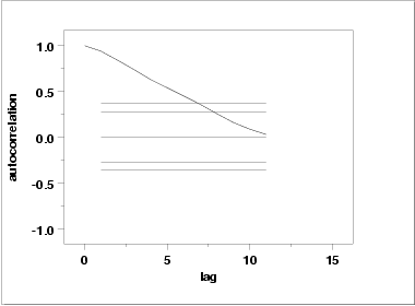
The lag 1 autocorrelation, which is generally the one of most interest, is 0.93. The critical values at the 5% level are -0.277 and 0.277. This indicates that the lag 1 autocorrelation is statistically significant, so there is strong evidence of non-randomness.
A common test for randomness is the
runs test.
|
||
| Distributional Analysis | Since we rejected the randomness assumption, the distributional tests are not meaningful. Therefore, these quantitative tests are omitted. We also omit Grubbs' outlier test since it also assumes the data are approximately normally distributed. | ||
| Univariate Report |
It is sometimes useful and convenient to summarize the above
results in a report.
Analysis for filter transmittance data
1: Sample Size = 50
2: Location
Mean = 2.001857
Standard Deviation of Mean = 0.00006
95% Confidence Interval for Mean = (2.001735,2.001979)
Drift with respect to location? = NO
3: Variation
Standard Deviation = 0.00043
95% Confidence Interval for SD = (0.000359,0.000535)
Change in variation?
(based on Levene's test on quarters
of the data) = NO
4: Distribution
Distributional tests omitted due to
non-randomness of the data
5: Randomness
Lag One Autocorrelation = 0.937998
Data are Random?
(as measured by autocorrelation) = NO
6: Statistical Control
(i.e., no drift in location or scale,
data are random, distribution is
fixed, here we are testing only for
normal)
Data Set is in Statistical Control? = NO
7: Outliers?
(Grubbs' test omitted) = NO
|
||