1. Exploratory Data Analysis
1.4. EDA Case Studies
1.4.2. Case Studies
1.4.2.7. Standard Resistor

1.4.2.7.2.

Graphical Output and Interpretation

Goal

The goal of this analysis is threefold:

1. Determine if the univariate model:
   \( Y_{i} = C + E_{i} \)

   is appropriate and valid.

2. Determine if the typical underlying assumptions for an "in control" measurement process are valid. These assumptions are:
   1. random drawings;
   2. from a fixed distribution;
   3. with the distribution having a fixed location; and
   4. the distribution having a fixed scale.
3. Determine if the confidence interval
   \( \bar{Y} \pm 2s/\sqrt{N} \)

   is appropriate and valid where s is the standard deviation of the original data.

4-Plot of Data

Interpretation

The assumptions are addressed by the graphics shown above:

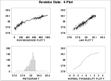
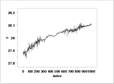
1. The run sequence plot (upper left) indicates significant shifts in both location and variation. Specifically, the location is increasing with time. The variability seems greater in the first and last third of the data than it does in the middle third.

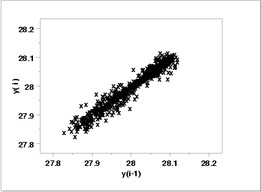
2. The lag plot (upper right) shows a significant non-random pattern in the data. Specifically, the strong linear appearance of this plot is indicative of a model that relates Y_t to Y_t-1.

3. The distributional plots, the histogram (lower left) and the normal probability plot (lower right), are not interpreted since the randomness assumption is so clearly violated.

The serious violation of the non-randomness assumption means that the univariate model

\( Y_{i} = C + E_{i} \)

is not valid. Given the linear appearance of the lag plot, the first step might be to consider a model of the type

\( Y_{i} = A_0 + A_1*Y_{i-1} + E_{i} \)

However, discussions with the scientist revealed the following:

1. the drift with respect to location was expected.

2. the non-constant variability was not expected.

The scientist examined the data collection device and determined that the non-constant variation was a seasonal effect. The high variability data in the first and last thirds was collected in winter while the more stable middle third was collected in the summer. The seasonal effect was determined to be caused by the amount of humidity affecting the measurement equipment. In this case, the solution was to modify the test equipment to be less sensitive to enviromental factors.

Simple graphical techniques can be quite effective in revealing unexpected results in the data. When this occurs, it is important to investigate whether the unexpected result is due to problems in the experiment and data collection, or is it in fact indicative of an unexpected underlying structure in the data. This determination cannot be made on the basis of statistics alone. The role of the graphical and statistical analysis is to detect problems or unexpected results in the data. Resolving the issues requires the knowledge of the scientist or engineer.

Individual Plots

Although it is generally unnecessary, the plots can be generated individually to give more detail. Since the lag plot indicates significant non-randomness, we omit the distributional plots.

Run Sequence Plot

Lag Plot