
1.4. EDA Case Studies
1.4.2. Case Studies
1.4.2.8. Heat Flow Meter 1
1.4.2.8.3. |
Quantitative Output and Interpretation |
      Sample size  = 195
      Mean         =   9.261460
      Median       =   9.261952
      Minimum      =   9.196848
      Maximum      =   9.327973
      Range        =   0.131126
      Stan. Dev.   =   0.022789
      Coefficient     Estimate     Stan. Error      t-Value
          B0           9.26699      0.3253E-02     2849.
          B1        -0.56412E-04    0.2878E-04     -1.960


      Residual Standard Deviation = 0.2262372E-01
      Residual Degrees of Freedom = 193
The slope parameter, B1, has a
t value of -1.96
which is (barely) statistically significant since it is essentially
equal to the 95 % level cutoff of -1.96. However, notice that the
value of the slope parameter estimate is -0.00056. This slope, even
though statistically significant, can essentially be considered zero.
      H0:  σ12 = σ22 = σ32 = σ42
      Ha:  At least one σi2 is not equal to the others.

      Test statistic:  T = 3.147
      Degrees of freedom:  k - 1 = 3
      Significance level:  α = 0.05
      Critical value:  Χ 21-α,k-1 = 7.815
      Critical region:  Reject H0 if T > 7.815
In this case, since the Bartlett test statistic of 3.147 is less than
the critical value at the 5 % significance level of 7.815, we conclude
that the variances are not significantly different in the
four intervals. That is, the assumption of constant scale is valid.
Another check is an autocorrelation plot that shows the autocorrelations for various lags. Confidence bands can be plotted at the 95 % and 99 % confidence levels. Points outside this band indicate statistically significant values (lag 0 is always 1).
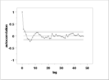
The lag 1 autocorrelation, which is generally the one of greatest interest, is 0.281. The critical values at the 5 % significance level are -0.140 and 0.140. This indicates that the lag 1 autocorrelation is statistically significant, so there is evidence of non-randomness.
A common test for randomness is the runs test.
      H0:  the sequence was produced in a random manner
      Ha:  the sequence was not produced in a random manner

      Test statistic:  Z = -3.2306
      Significance level:  α = 0.05
      Critical value:  Z1-α/2 = 1.96
      Critical region:  Reject H0 if |Z| > 1.96
The value of the test statistic is less than -1.96, so we reject the
null hypothesis at the 0.05 significant level and conclude that the
data are not random.
Although the autocorrelation plot and the runs test indicate some mild non-randomness, the violation of the randomness assumption is not serious enough to warrant developing a more sophisticated model. It is common in practice that some of the assumptions are mildly violated and it is a judgement call as to whether or not the violations are serious enough to warrant developing a more sophisticated model for the data.
A quantitative enhancement to the probability plot is the correlation coefficient of the points on the probability plot. For this data set the correlation coefficient is 0.996. Since this is greater than the critical value of 0.987 (this is a tabulated value), the normality assumption is not rejected.
Chi-square and Kolmogorov-Smirnov goodness-of-fit tests are alternative methods for assessing distributional adequacy. The Wilk-Shapiro and Anderson-Darling tests can be used to test for normality. The results of the Anderson-Darling test follow.
      H0:  the data are normally distributed
      Ha:  the data are not normally distributed

      Adjusted test statistic:  A 2 = 0.129
      Significance level:  α = 0.05
      Critical value:  0.787
      Critical region:  Reject H0 if A 2 > 0.787
The Anderson-Darling test also does not reject the normality
assumption because the test statistic, 0.129, is less than the
critical value at the 5 % significance level of 0.787.
      H0:  there are no outliers in the data
      Ha:  the maximum value is an outlier

      Test statistic:  G = 2.918673
      Significance level:  α = 0.05
      Critical value for an upper one-tailed test:  3.597898
      Critical region:  Reject H0 if G > 3.597898
For this data set, Grubbs' test does not detect any outliers at
the 0.05 significance level.
-
\( Y_{i} = 9.26146 + E_{i} \)
 Analysis for heat flow meter data

 1: Sample Size                           = 195

 2: Location
    Mean                                  = 9.26146
    Standard Deviation of Mean            = 0.001632
    95 % Confidence Interval for Mean     = (9.258242,9.264679)
    Drift with respect to location?       = NO

 3: Variation
    Standard Deviation                    = 0.022789
    95 % Confidence Interval for SD       = (0.02073,0.025307)
    Drift with respect to variation?
    (based on Bartlett's test on quarters
    of the data)                          = NO

 4: Randomness
    Autocorrelation                       = 0.280579
    Data are Random?
      (as measured by autocorrelation)    = NO

 5: Data are Normal?
      (as tested by Anderson-Darling)     = YES
      (as tested by Normal PPCC)          = YES

 6: Statistical Control
    (i.e., no drift in location or scale,
    data are random, distribution is
    fixed, here we are testing only for
    fixed normal)
    Data Set is in Statistical Control?   = YES

 7: Outliers?
    (as determined by Grubbs' test)        = NO
