6.1.6. What is Process Capability?

6. Process or Product Monitoring and Control
6.1. Introduction

6.1.6. What is Process Capability?

Process capability compares the output of an in-control process to the specification limits by using capability indices. The comparison is made by forming the ratio of the spread between the process specifications (the specification "width") to the spread of the process values, as measured by 6 process standard deviation units (the process "width").

Process Capability Indices

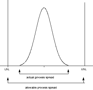
A process capability index uses both the process variability and the process specifications to determine whether the process is "capable"

We are often required to compare the output of a stable process with the process specifications and make a statement about how well the process meets specification. To do this we compare the natural variability of a stable process with the process specification limits.

A process where almost all the measurements fall inside the specification limits is a capable process. This can be represented pictorially by the plot below:

Diagram demonstrating a capable process

There are several statistics that can be used to measure the capability of a process: $C_p$, $C_{pk}$, and $C_{pm}$.

Most capability indices estimates are valid only if the sample size used is "large enough". Large enough is generally thought to be about 50 independent data values.

The $C_p$, $C_{pk}$, and $C_{pm}$ statistics assume that the population of data values is normally distributed. Assuming a two-sided specification, if $\mu$ and $\sigma$ are the mean and standard deviation, respectively, of the normal data and $\mbox{USL}$, $\mbox{LSL}$, and $T$ are the upper and lower specification limits and the target value, respectively, then the population capability indices are defined as follows.

Definitions of various process capability indices

$$ C_{p} = \frac{\mbox{USL} - \mbox{LSL}} {6\sigma} $$

$$C_{pk} = \min{\left[ \frac{\mbox{USL} - \mu} {3\sigma}, \frac{\mu - \mbox{LSL}} {3\sigma}\right]} $$

$$ C_{pm} = \frac{\mbox{USL} - \mbox{LSL}} {6\sqrt{\sigma^2 + (\mu - T)^2}} $$

Sample estimates of capability indices

Sample estimators for these indices are given below. (Estimators are indicated with a "hat" over them).

$$ \hat{C}_{p} = \frac{\mbox{USL} - \mbox{LSL}} {6s} $$

$$ \hat{C}_{pk} = \min{\left[ \frac{\mbox{USL} - \bar{x}} {3s}, \frac{\bar{x} - \mbox{LSL}} {3s}\right]} $$

$$ \hat{C}_{pm} = \frac{\mbox{USL} - \mbox{LSL}} {6\sqrt{s^2 + (\bar{x} - T)^2}} $$

The estimator for $C_{pk}$ can also be expressed as $C_{pk} = C_p(1-k)$, where $k$ is a scaled distance between the midpoint of the specification range, $m$, and the process mean, $\mu$.

Denote the midpoint of the specification range by $m = (\mbox{USL} + \mbox{LSL})/2$. The distance between the process mean, $\mu$, and the optimum, which is $m$, is $\mu - m$, where $m \le \mu \le \mbox{LSL}$. The scaled distance is $$ k = \frac{|m - \mu|} {(\mbox{USL} - \mbox{LSL})/2}, \;\;\;\;\;\; 0 \le k \le 1 \, .$$ (The absolute sign takes care of the case when $\mbox{LSL} \le \mu \le m$). To determine the estimated value, $\hat{k}$, we estimate $\mu$ by $\bar{x}$. Note that $\bar{x} \le \mbox{USL}$.

The estimator for the $C_p$ index, adjusted by the $k$ factor, is $$ \hat{C}_{pk} = \hat{C}_{p}(1 - \hat{k}) \, . $$ Since $0 \le k \le 1$, it follows that $\hat{C}_{pk} \le \hat{C}_{p}$.

Plot showing $C_p$ for varying process widths

To get an idea of the value of the $C_p$ statistic for varying process widths, consider the following plot.

4 plots showing the value of Cp for varying process widths

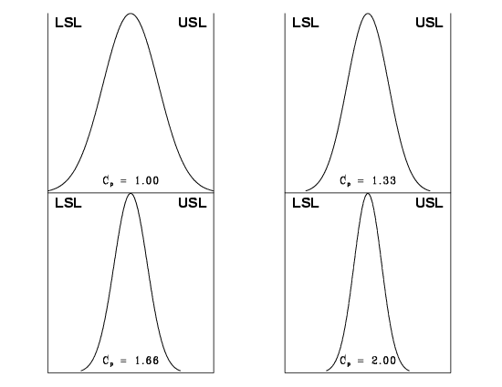
This can be expressed numerically by the table below:

Translating capability into "rejects"

$\mbox{USL} - \mbox{LSL}$	$6 \sigma$	$8 \sigma$	$10 \sigma$	$12 \sigma$
$C_p$	1.00	1.33	1.66	2.00
Rejects	0.27 %	64 ppm	0.6 ppm	2 ppb
% of spec used	100	75	60	50

where ppm = parts per million and ppb = parts per billion. Note that the reject figures are based on the assumption that the distribution is centered at $\mu$.

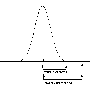
We have discussed the situation with two spec. limits, the $\mbox{USL}$ and $\mbox{LSL}$. This is known as the bilateral or two-sided case. There are many cases where only the lower or upper specifications are used. Using one spec limit is called unilateral or one-sided. The corresponding capability indices are

One-sided specifications and the corresponding capability indices

$$ C_{pu} = \frac{\mbox{allowable upper spread}} {\mbox{actual upper spread}} = \frac{\mbox{USL} - \mu} {3\sigma} $$ and $$ C_{pl} = \frac{\mbox{allowable lower spread}} {\mbox{actual lower spread}} = \frac{\mu - \mbox{LSL}} {3\sigma} \, , $$ where $\mu$ and $\sigma$ are the process mean and standard deviation, respectively.

Estimators of $C_{pu}$ and $C_{pl}$ are obtained by replacing $\mu$ and $\sigma$ by $\bar{x}$ and $s$, respectively. The following relationship holds $$ C_p = \frac{C_{pu} + C_{pl}}{2} \, . $$ This can be represented pictorially by

Graph demonstrating upper actual and allowable upper spread

Note that we also can write:

$$ C_{pk} = \mbox{min}(C_{pl}, \, C_{pu}) \, . $$

Confidence Limits For Capability Indices

Confidence intervals for indices

Assuming normally distributed process data, the distribution of the sample $\hat{C}_p$ follows from a Chi-square distribution and $\hat{C}_{pu}$ and $\hat{C}_{pl}$ have distributions related to the non-central t distribution. Fortunately, approximate confidence limits related to the normal distribution have been derived. Various approximations to the distribution of $\hat{C}_{pk}$ have been proposed, including those given by Bissell (1990), and we will use a normal approximation.

The resulting formulas for $100(1-\alpha) \%$ confidence limits are given below.

Confidence Limits for $C_p$ are $$ Pr\{\hat{C}_{p}(L_1) \le C_p \le \hat{C}_{p}(L_2)\} = 1 - \alpha \, ,$$ where $$ \begin{eqnarray} L_1 & = & \sqrt{\frac{\chi^2_{\alpha/2, \, \nu}}{\nu}} \, , \\ & & \\ L_2 & = & \sqrt{\frac{\chi^2_{1-\alpha/2, \, \nu}}{\nu}} \, , \end{eqnarray}$$ and $\nu = $ degrees of freedom.

Confidence Intervals for $C_{pu}$ and $C_{pl}$

Approximate $100(1-\alpha)$ % confidence limits for $C_{pu}$ with sample size $n$ are: $$ C_{pu}(lower) = \hat{C}_{pu} - z_{1-\beta}\sqrt{\frac{1}{9n} + \frac{\hat{C}_{pu}^{2}}{2(n-1)}} $$ and

$$ C_{pu}(upper) = \hat{C}_{pu} + z_{1-\alpha}\sqrt{\frac{1}{9n} + \frac{\hat{C}_{pu}^{2}}{2(n-1)}} \, ,$$ with $z$ denoting the percent point function of the standard normal distribution. If $\beta$ is not known, set it to $\alpha$.

Limits for $C_{pl}$ are obtained by replacing $\hat{C}_{pu}$ by $\hat{C}_{pl}$.

Confidence Interval for $C_{pk}$

Zhang et al. (1990) derived the exact variance for the estimator of $C_{pk}$ as well as an approximation for large $n$. The reference paper is Zhang, Stenback and Wardrop (1990), "Interval Estimation of the process capability index," Communications in Statistics: Theory and Methods, 19(21), 4455-4470.

The variance is obtained as follows.

Let

$$ c = \sqrt{n}\left[\mu - (\mbox{USL} + \mbox{LSL})/2\right]\sigma $$ $$ d = (\mbox{USL} - \mbox{LSL})/\sigma $$ $$ \Phi(-c) = \int_{-inf}^{-c}{\frac{1}{\sqrt{2\pi}}\exp{-5z^2}dz} \, .$$ Then

$$ Var(\hat{C}_{pk}) $$ $$ = (d^2/36)(n-1)(n-3) $$ $$ -(d/9\sqrt{n})(n-1)(n-3)\{\sqrt{2\pi}\exp{(-c^2/2)} + c[1 - 2\Phi(-c)]\} $$ $$ +[(1/9)(n-1)/(n(n-3))](1+c^2) $$ $$ -[(n-1)/(72n)]\{\frac{\Gamma((n-2)/2)}{\Gamma((n-1)/2)}\}^2 $$ $$ *\{d\sqrt{n} - 2\sqrt{2\pi}\exp{(-c^2/2)} - 2c[1 - 2\Phi(-c)]\}^2 \, .$$ Their approximation is given by:

$$ Var(\hat{C}_{pk}) = \frac{n-1}{n-3} - 0.5\{\frac{\Gamma((n-2)/2)}{\Gamma((n-1)/2)}\}^2 \, , $$ where

$$ n \ge 25, \,\,\,\,\,\, 0.75 \le C_{pk} \le 4, \,\,\,\,\,\, |c| \le 100, \,\,\,\,\,\, \mbox{ and } \,\,\,\,\,\, d \le 24 \, .$$ The following approximation is commonly used in practice $$ C_{pk} = \hat{C}_{pk} \pm z_{1-\alpha/2}\sqrt{\frac{1}{9n} + \frac{\hat{C}_{pk}^{2}}{2(n-1)}} \, . $$ It is important to note that the sample size should be at least 25 before these approximations are valid. In general, however, we need $n \ge 100$ for capability studies. Another point to observe is that variations are not negligible due to the randomness of capability indices.

Capability Index Example

An example

For a certain process the $\mbox{USL} = 20$ and the $\mbox{LSL} = 8$. The observed process average, $\bar{x} \ge 16$, and the standard deviation, $s = 2$. From this we obtain $$ \hat{C}_{p} = \frac{\mbox{USL} - \mbox{LSL}} {6s} = \frac{20 - 8} {6(2)} = 1.0 \, . $$ This means that the process is capable as long as it is located at the midpoint, $m = (\mbox{USL} + \mbox{LSL})/2 = 14$.

But it doesn't, since $\bar{x} \ge 16$. The $\hat{k}$ factor is found by $$ \hat{k} = \frac{|m - \bar{x}|} {(\mbox{USL} - \mbox{LSL})/2} = \frac{2} {6} = 0.3333 $$ and $$ \hat{C}_{pk} = \hat{C}_{p}(1-\hat{k}) = 0.6667 \, .$$ We would like to have $\hat{C}_{pk}$ at least 1.0, so this is not a good process. If possible, reduce the variability or/and center the process. We can compute the $\hat{C}_{pu}$ and $\hat{C}_{pl}$ using $$ \hat{C}_{pu} = \frac{\mbox{USL} - \bar{x}} {3s} = \frac{20 - 16} {3(2)} = 0.6667 $$ and $$ \hat{C}_{pl} = \frac{\bar{x} - \mbox{LSL}} {3s} = \frac{16 - 8} {3(2)} = 1.3333 \, . $$ From this we see that the $\hat{C}_{pu}$, which is the smallest of the above indices, is 0.6667. Note that the formula $\hat{C}_{pk} = \hat{C}_{p}(1 - \hat{k})$ is the algebraic equivalent of the $\mbox{min}(\hat{C}_{pu}, \, \hat{C}_{pl})$ definition.

What happens if the process is not approximately normally distributed?

What you can do with non-normal data

The indices that we considered thus far are based on normality of the process distribution. This poses a problem when the process distribution is not normal. Without going into the specifics, we can list some remedies.

Transform the data so that they become approximately normal. A popular transformation is the Box-Cox transformation
Use or develop another set of indices, that apply to nonnormal distributions. Non-parameteric versions (Pearn, Tai, Hsiao, and Ao (2014) and Chen and Ding (2001)) of the $C_{p}$, $C_{pk}$, and $C_{pm}$ capability indices are denoted by $C_{np}$, $C_{npk}$, and $C_{npm}$. Estimators for these non-parameteric capability indices are calculated by
where $p(0.99855)$ is the 99.865th percentile of the data and $p(0.00135)$ is the 0.135th percentile of the data. The use of these percentiles is justified to mimic the coverage of ±3 standard deviations for the normal distribution. Note that some sources may use 99% coverage. For example, the $C_{npk}$ statistic may be given as
where $p(0.995)$ is the 99.5th percentile of the data and $p(0.005)$ is the 0.5th percentile of the data.

For additional information on nonnormal distributions, see Johnson and Kotz (1993).

There is, of course, much more that can be said about the case of nonnormal data. However, if a Box-Cox transformation can be successfully performed, one is encouraged to use it.