6. Process or Product Monitoring and Control
6.4. Introduction to Time Series Analysis

6.4.2.

What are Moving Average or Smoothing Techniques?

Smoothing data removes random variation and shows trends and cyclic components

Inherent in the collection of data taken over time is some form of random variation. There exist methods for reducing of canceling the effect due to random variation. An often-used technique in industry is "smoothing". This technique, when properly applied, reveals more clearly the underlying trend, seasonal and cyclic components.

There are two distinct groups of smoothing methods 

• Averaging Methods
• Exponential Smoothing Methods

Taking averages is the simplest way to smooth data

We will first investigate some averaging methods, such as the "simple" average of all past data.

A manager of a warehouse wants to know how much a typical supplier delivers in 1000 dollar units. He/she takes a sample of 12 suppliers, at random, obtaining the following results:

Supplier	Amount	Supplier	Amount
1	9	7	11
2	8	8	7
3	9	9	13
4	12	10	9
5	9	11	11
6	12	12	10

The computed mean or average of the data = 10. The manager decides to use this as the estimate for expenditure of a typical supplier.

Is this a good or bad estimate? 

Mean squared error is a way to judge how good a model is

We shall compute the "mean squared error":

• The "error" = true amount spent minus the estimated amount.
• The "error squared" is the error above, squared.
• The "SSE" is the sum of the squared errors.
• The "MSE" is the mean of the squared errors.

MSE results for example

The results are: Error and Squared Errors

The estimate = 10

Supplier	$	Error	Error Squared
1	9	-1	1
2	8	-2	4
3	9	-1	1
4	12	2	4
5	9	-1	1
6	12	2	4
7	11	1	1
8	7	-3	9
9	13	3	9
10	9	-1	1
11	11	1	1
12	10	0	0

The SSE = 36 and the MSE = 36/12 = 3.

Table of MSE results for example using different estimates

So how good was the estimator for the amount spent for each supplier? Let us compare the estimate (10) with the following estimates: 7, 9, and 12. That is, we estimate that each supplier will spend $7, or $9 or $12.

Performing the same calculations we arrive at:

Estimator	7	9	10	12
SSE	144	48	36	84
MSE	12	4	3	7

The estimator with the smallest MSE is the best. It can be shown mathematically that the estimator that minimizes the MSE for a set of random data is the mean.

Table showing squared error for the mean for sample data

Next we will examine the mean to see how well it predicts net income over time.

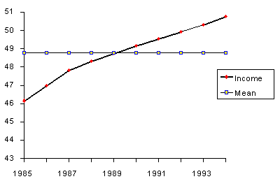
The next table gives the income before taxes of a PC manufacturer between 1985 and 1994.

Year	$ (millions)	Mean	Error	Squared Error
1985	46.163	48.676	-2.513	6.313
1986	46.998	48.676	-1.678	2.814
1987	47.816	48.676	-0.860	0.739
1988	48.311	48.676	-0.365	0.133
1989	48.758	48.676	0.082	0.007
1990	49.164	48.676	0.488	0.239
1991	49.548	48.676	0.872	0.761
1992	48.915	48.676	0.239	0.057
1993	50.315	48.676	1.639	2.688
1994	50.768	48.676	2.092	4.378

The MSE = 1.8129.

The mean is not a good estimator when there are trends

The question arises: can we use the mean to forecast income if we suspect a trend? A look at the graph below shows clearly that we should not do this.

Average weighs all past observations equally

In summary, we state that

1. The "simple" average or mean of all past observations is only a useful estimate for forecasting when there are no trends. If there are trends, use different estimates that take the trend into account.

2. The average "weighs" all past observations equally. For example, the average of the values 3, 4, 5 is 4. We know, of course, that an average is computed by adding all the values and dividing the sum by the number of values. Another way of computing the average is by adding each value divided by the number of values, or
   3/3 + 4/3 + 5/3 = 1 + 1.3333 + 1.6667 = 4.

   The multiplier 1/3 is called the weight. In general:

   $$ \bar{x} = \frac{1} {n} \sum_{i=1}^{n}{x_i} = \left ( \frac{1} {n} \right ) x_1 + \left ( \frac{1} {n} \right ) x_2 \, + \, ... \, + \, \left ( \frac{1} {n} \right ) x_n \, . $$

   The \( \left ( \frac{1} {n} \right ) \) are the weights and, of course, they sum to 1.