4. Process Modeling
4.6. Case Studies in Process Modeling
4.6.2. Alaska Pipeline

4.6.2.5.

Weighting to Improve Fit

Weighting

Another approach when the assumption of constant standard deviation of the errors (i.e. homogeneous variances) is violated is to perform a weighted fit. In a weighted fit, we give less weight to the less precise measurements and more weight to more precise measurements when estimating the unknown parameters in the model.

Fit for Estimating Weights

For the pipeline data, we chose approximate replicate groups so that each group has four observations (the last group only has three). This was done by first sorting the data by the predictor variable and then taking four points in succession to form each replicate group.

Using the power function model with the data for estimating the weights, the following results for the fit of ln(variances) against ln(means) for the replicate groups were generated.

Parameter     Estimate    Stan. Dev    t Value
B0            -3.18451       0.8265       -3.9
B1             1.69001       0.2344        7.2

Residual standard deviation = 0.85612
Residual degrees of freedom = 25

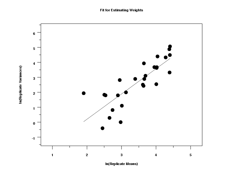The numerical fitting results and the plot of the replicate variances against the replicate means shows that a linear fit provides a reasonable fit with an estimated slope of 1.69.

We used an estimate of 1.5 for the exponent in the weighting function.

Residual Plot for Weight Function

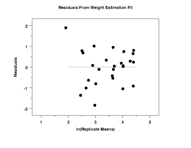
The residual plot from the fit to determine an appropriate weighting function reveals no obvious problems.

Numerical Results from Weighted Fit

The weighted fit of the model that relates the field measurements to the lab measurements is shown below.

Parameter     Estimate    Stan. Dev    t Value
B0             2.35234      0.54312        4.3
B1             0.80636      0.02265       35.6

Residual standard deviation = 0.36459
Residual degrees of freedom = 105

The resulting slope and intercept are 0.81 and 2.35, respectively. These are compared to a slope of 0.73 and an intercept of 4.99 in the original model.

Plot of Predicted Values

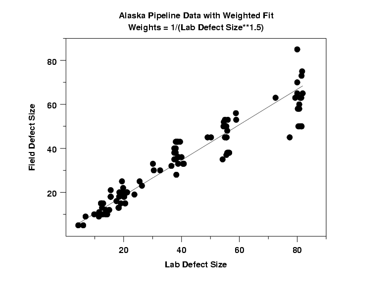
The plot of the predicted values with the data indicates a good fit.

Diagnostic Plots of Weighted Residuals

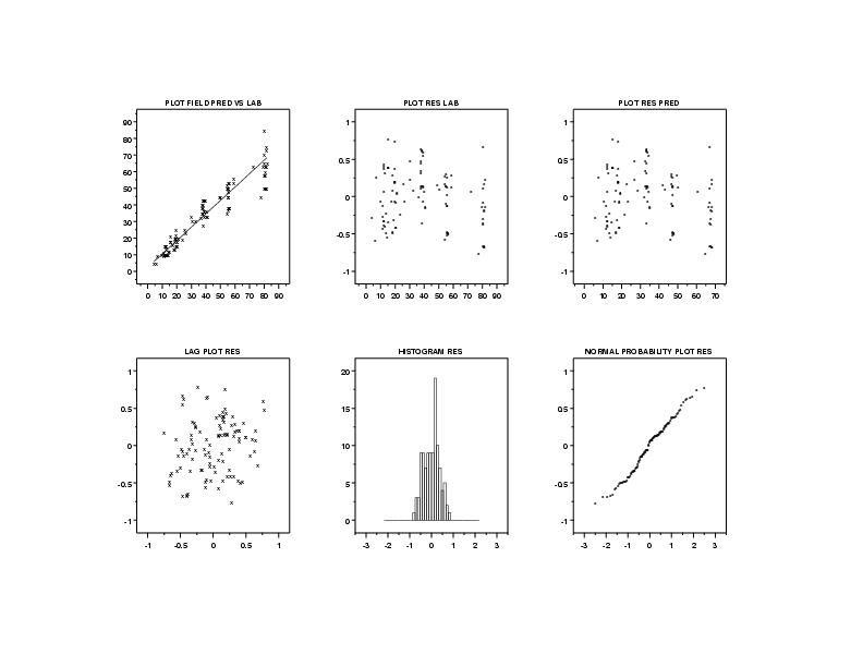
We need to verify that the weighting did not result in the other regression assumptions being violated. A 6-plot, after weighting the residuals, indicates that the regression assumptions are satisfied.

Plot of Weighted Residuals vs Lab Defect Size

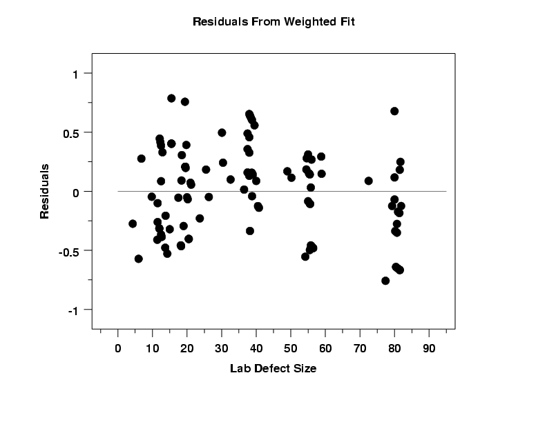
In order to check the assumption of homogeneous variances for the errors in more detail, we generate a full sized plot of the weighted residuals versus the predictor variable. This plot suggests that the errors now have homogeneous variances.