5.
Process Improvement
5.5.
Advanced topics
5.5.3.
How do you optimize a process?
5.5.3.1.
Single response case
5.5.3.1.4.
|
Single response: Optimization when there is adequate quadratic fit
|
|
|
Regions where quadratic models or even cubic models are needed
occur in many instances in industry
|
After a few steepest ascent (or descent) searches, a first-order model
will eventually lead to no further improvement or it will exhibit lack
of fit. The latter case typically occurs when operating conditions
have been changed to a region where there are quadratic (second-order)
effects present in the response. A second-order polynomial can be
used as a local approximation of the response in a small region where,
hopefully, optimal operating conditions exist. However, while a
quadratic fit is appropriate in most of the cases in industry, there
will be a few times when a quadratic fit will not be sufficiently
flexible to explain a given response. In such cases, the analyst
generally does one of the following:
- Uses a transformation of Y or the \( X_{i} \)'s
to improve the fit.
- Limits use of the model to a smaller region in which the model
does fit.
- Adds other terms to the model.
|
|
|
Procedure: obtaining the estimated optimal operating conditions
|
Second-
order polynomial model
|
Once a linear model exhibits lack of fit or when significant curvature
is detected, the experimental design used in Phase I (recall that a
2k-p factorial experiment might be
used) should be augmented with axial runs on each factor to form what
is called a central composite design. This experimental design
allows estimation of a second-order polynomial of the form
\[ \hat{Y} = b_{0} + \sum_{i=1}^{k}{b_{i}x_{i}} +
\sum_{i=1}^{k}{b_{ii}x_{i}^{2}} +
\sum_{i < j}^{k}{\sum_{j=1}^{k}{b_{ij}x_{i}x_{j}}}
\]
|
|
Steps to find optimal operating conditions
|
If the corresponding analysis of variance table indicates no lack of
fit for this model, the engineer can proceed to determine the estimated
optimal operating conditions.
- Using some graphics software, obtain a contour plot of the
fitted response. If the number of factors (k) is
greater than 2, then plot contours in all planes corresponding to
all the possible pairs of factors. For k greater
than, say, 5, this could be too cumbersome (unless the graphic
software plots all pairs automatically). In such a case, a
"canonical analysis" of the surface is recommended (see
Technical Appendix 5D).
- Use an optimization solver to maximize or minimize (as desired)
the estimated response \( \hat{Y} \).
- Perform a confirmation experiment at the estimated optimal
operating conditions given by the solver in step 2.
|
|
Chemical experiment example
|
We illustrate these steps using the
chemical
experiment discussed previously. For a technical description of a
formula that provides the coordinates of the stationary point of the
surface, see Technical
Appendix 5C.
|
|
|
Example: Second Phase Optimization of Chemical Process
|
|
Experimental results for axial runs
|
Recall that in the chemical experiment, the
ANOVA table,
obtained from using an experiment run around the coordinates
X1 = 189.5, X2 = 350,
indicated significant curvature effects. Augmenting the
22 factorial experiment with axial runs at
\( \pm \alpha = \pm \sqrt{2} \)
to achieve a rotatable central composite experimental design, the
following experimental results were obtained:
|
x1
|
x2
|
X1
|
X2
|
Y (= yield)
|
|
-1.414
|
0
|
147.08
|
350
|
72.58
|
|
+1.414
|
0
|
231.92
|
350
|
37.42
|
|
0
|
-1.414
|
189.5
|
279.3
|
54.63
|
|
0
|
+1.414
|
189.5
|
420.7
|
54.18
|
(The reader can download the data as a
text file.)
|
|
ANOVA table
|
The ANOVA table corresponding to a cubic model with an interaction term (contained
in the quadratic sum-of-squares partition) is
               SUM OF            MEAN      F
SOURCE        SQUARES   DF      SQUARE   VALUE  PROB > F

MEAN          51418.2    1     51418.2
Linear         1113.7    2       556.8    5.56    0.024
Quadratic       768.1    3       256.0    7.69    0.013
Cubic             9.9    2         5.0    0.11    0.897

RESIDUAL        223.1    5        44.6
TOTAL         53533.0   13
|
|
Lack-of-fit tests and auxillary diagnostic statistics
|
From the ANOVA table, the linear and quadratic effects are significant. The
lack-of-fit tests and auxiliary diagnostic statistics for linear, quadratic,
and cubic models are:
              SUM OF             MEAN      F
MODEL        SQUARES      DF    SQUARE   VALUE  PROB > F

Linear         827.9       6     138.0    3.19    0.141
Quadratic       59.9       3      20.0    0.46    0.725
Cubic           49.9       1      49.9    1.15    0.343

PURE ERROR     173.2       4      43.3

              ROOT                ADJ       PRED
MODEL         MSE      R-SQR     R-SQR      R-SQR    PRESS

Linear       10.01    0.5266    0.4319     0.2425    1602.02
Quadratic     5.77    0.8898    0.8111     0.6708     696.25
Cubic         6.68    0.8945    0.7468    -0.6393    3466.71
The quadratic model has a larger p-value for the lack of fit
test, higher adjusted R2, and a lower PRESS statistic; thus
it should provide a reliable model. The fitted quadratic equation, in
coded units, is
\( \hat{Y} = 72.0 - 11.78x_{1} + 0.74x_{2} - 7.25x_{1}^{2} -
7.55x_{2}^{2} - 4.85x_{1}x_{2} \)
|
|
|
Step 1:
|
|
Contour plot of the fitted response function
|
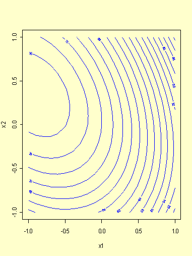
A contour plot of this function (Figure 5.5) shows that it appears to
have a single optimum point in the region of the experiment (this
optimum is calculated below to be (-0.9285, 0.3472), in coded
x1, x2 units, with a
predicted response value of 77.59).

FIGURE 5.5: Contour Plot of the Fitted Response in the Example
|
|
3D plot of the fitted response function
|
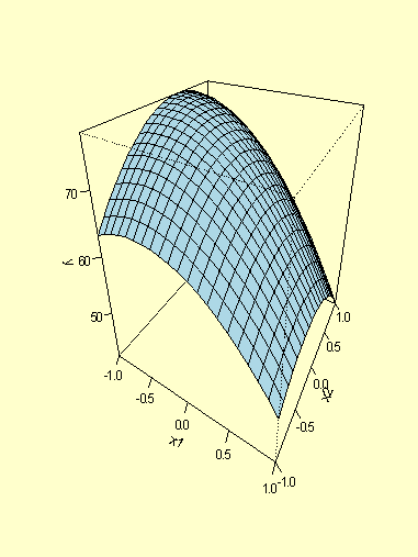
Since there are only two factors in this example, we can also obtain a
3D plot of the fitted response against the two factors (Figure 5.6).

FIGURE 5.6: 3D Plot of the Fitted Response in the Example
|
|
|
Step 2:
|
|
Optimization point
|
An optimization routine was used to maximize \( \hat{Y} \).
The results are \( X_{1}^{*} = 161.64^{\circ}C \),
\( X_{2}^{*} = 367.32 \)
minutes. The estimated yield at the optimal point is
\( \hat{Y}(X^{*}) = 77.59 \)%,
|
|
|
Step 3:
|
|
Confirmation experiment
|
A confirmation experiment was conducted by the process engineer at
settings X1 = 161.64,
X2 = 367.32.
The observed response was \( \hat{Y}(X^{*}) = 76.5 \)%,
which is satisfactorily close to the estimated optimum.
|
|
|
|
|
|
Technical Appendix 5C: Finding the Factor Settings for the
Stationary Point of a Quadratic Response
|
|
How to find the maximum or minimum point for a
quadratic response
|
- Rewrite the fitted equation using matrix notation as
\( \hat{Y}(x) = b_{0} + b'x + x'Bx \)
where b' = (b1,
b2, ..., bk)
denotes a vector of first-order parameter estimates,
\(
B = \left(
\begin{array}{cccc}
b_{11} & b_{12}/2 & \cdots & b_{ik}/2 \\
& b_{22} & & \\
& & \ddots & \vdots \\
\mbox{symmetric} & & & b_{kk}
\end{array}
\right)
\)
is a matrix of second-order parameter estimates and
x' = (x1,
x2, ..., xk)
is the vector of controllable factors. Notice that the
off-diagonal elements of B are equal to half
the two-factor interaction coefficients.
- Equating the partial derivatives of \( \hat{Y} \)
with respect to x to zeroes and solving the
resulting system of equations, the coordinates of the
stationary point of the response are given by
\( x^{*} = -\frac{1}{2}B^{-1}b \)
|
|
Nature of the stationary point is determined by B
|
The nature of the stationary point (whether it is a point of maximum
response, minimum response, or a saddle point) is determined by the
matrix B. The two-factor interactions do not, in
general, let us "see" what type of point x*
is. One thing that can be said is that if the diagonal elements of
B (bii) have mixed signs,
x* is a saddle point. Otherwise, it is
necessary to look at the characteristic roots or eigenvalues of
B to see whether B is "positive definite"
(so x* is a point of minimum response) or
"negative definite" (the case in which x*
is a point of maximum response). This task is easier if the two-factor
interactions are "eliminated" from the fitted equation as is described
in Technical Appendix 5D.
|
|
|
Example: computing the stationary point, Chemical Process
experiment
|
|
Example of computing the stationary point
|
The fitted quadratic equation in the chemical experiment discussed in
Section 5.5.3.1.1 is, in coded units,
\( \hat{Y} = 72.0 - 11.78x_{1} + 0.74x_{2} - 7.25x_{1}^{2} -
7.55x_{2}^{2} - 4.85x_{1}x_{2} \)
from which we obtain b' = (-11.78, 0.74),
\( B =
\left(
\begin{array}{cc}
-7.25 & -2.2425 \\
-2.425 & -7.55
\end{array}
\right)
\) ;
\( B^{-1} =
\left(
\begin{array}{cc}
-0.1545 & 0.0496 \\
0.0496 & -0.1483
\end{array}
\right)
\)
and
\( x^{*} = -\frac{1}{2}
\left(
\begin{array}{cc}
-0.1545 & 0.0496 \\
0.0496 & -0.1483
\end{array}
\right)
\left(
\begin{array}{c}
-11.78 \\
0.74
\end{array}
\right)
=
\left(
\begin{array}{c}
-0.9285 \\
0.3472 \\
\end{array}
\right)
\)
Transforming back to the original units of measurement, the coordinates
of the stationary point are
\( X^{*} =
\left(
\begin{array}{c}
161.64^{\circ}C \\
367.36 \mbox{ minutes}
\end{array}
\right)
\)
The predicted response at the stationary point is
\( \hat{Y}(X^{*}) = 77.59% \).
|
|
|
Technical Appendix 5D: "Canonical Analysis" of Quadratic
Responses
|
|
Case for a single controllable response
|
Whether the stationary point X* represents a
point of maximum or minimum response, or is just a saddle point, is
determined by the matrix of second-order coefficients, B.
In the simpler case of just a single controllable factor
(k=1), B is a scalar proportional to the
second derivative of
\( \hat{Y}(x) \)
with respect to x. If
\( d^{2}\hat{Y}/dx^{2} \)
is positive, recall from calculus that the function
\( \hat{Y}(x) \)
is convex ("bowl shaped") and x*
is a point of minimum response.
|
|
Case for multiple controllable responses not so easy
|
Unfortunately, the multiple factor case (k>1) is not so easy
since the two-factor interactions (the off-diagonal elements of
B) obscure the picture of what is going on. A
recommended procedure for analyzing whether
B is "positive definite" (we have a minimum) or
"negative definite" (we have a maximum) is to rotate the axes
x1, x2, ...,
xk so that the two-factor interactions disappear.
It is also customary (Box
and Draper, 1987; Khuri and
Cornell, 1987; Myers and
Montgomery, 1995) to translate the origin of coordinates to the
stationary point so that the intercept term is eliminated from the
equation of \( \hat{Y}(x) \).
This procedure is called the canonical analysis of
\( \hat{Y}(x) \).
|
|
|
Procedure: Canonical Analysis
|
|
Steps for performing the canonical analysis
|
- Define a new axis
z = x - x*
(translation step). The fitted equation becomes
\( \hat{Y}(z) = \hat{Y}(x^{*}) + z'Bz \)
- Define a new axis w = E'z,
with E'BE = D
and D a diagonal matrix to be defined (rotation
step). The fitted equation becomes
\( \hat{Y}(w) = \hat{Y}(x^{*}) + w'Dw \)
This is the so-called canonical form of the model. The
elements on the diagonal of D,
λi
(i = 1, 2, ..., k)
are the eigenvalues of B. The columns of
E', ei,
are the orthonormal eigenvectors of B,
which means that the ei satisfy
(B -
λi)ei = 0,
\( e_{i}^{'}e_{i} \)
= 0 for i ≠ j, and
\( e_{i}^{'}e_{i} \)
= 1.0.
- If all the λi are negative,
x* is a point of maximum response. If
all the λi are positive,
x* is a point of minimum response.
Finally, if the λi are of
mixed signs, the response is a saddle function and
x* is the saddle point.
|
|
Eigenvalues that are approximately zero
|
If some λi
≈ 0, the fitted ellipsoid
\[ \hat{Y}(w) = \hat{Y}(x^{*}) +
\sum_{i=1}^{k}{\lambda_{i}w_{i}^{2}} \]
is elongated (i.e., it is flat) along the direction of the
wi axis. Points along the
wi axis will have an estimated response close
to optimal; thus the process engineer has flexibility in choosing
"good" operating conditions. If two eigenvalues (say
λi and
λj)
are close to zero, a plane in the
(wi, wj)
coordinates will have close to optimal operating conditions, etc.
|
|
Canonical analysis typically performed by software
|
Software is available to compute the eigenvalues
λi and
the orthonormal eigenvectors ei;
thus there is no need to do a canonical analysis by hand.
|
|
|
Example: Canonical Analysis of Yield Response in Chemical
Experiment
|
|
B matrix for this example
|
Let us return to the chemical experiment
example to illustrate the method. Keep
in mind that when the number of factors is small (e.g., k=2
as in this example) canonical analysis is not recommended in practice
since simple contour plotting will provide sufficient information. The
fitted equation of the model yields
\( B =
\left(
\begin{array}{cc}
-7.25 & -2.2425 \\
-2.425 & -7.55
\end{array}
\right)
\)
|
|
Compute the eigenvalues and find the orthonormal eigenvectors
|
To compute the eigenvalues λi,
we have to find all roots of the expression that results from equating
the determinant of B - λiI to
zero. Since B is symmetric and has real coefficients, there
will be k real roots
λi, i = 1, 2, ..., k.
To find the orthonormal eigenvectors, solve the simultaneous equations
\( (B - \lambda_{i}I)e_{i} = 0 \)
and \( e_{i}^{'}e_{i} = 1 \).
|
|
Canonical analysis results
|
The results of the canonical analysis are as follows:
                                     Eigenvectors
              Eigenvalues         X1               X2

                -4.973187        0.728460       -0.685089
                -9.827317        0.685089        0.728460
Notice that the eigenvalues are the two roots of
\( \mbox{det}(B - \lambda I) = (-7.25 - \lambda)(-7.55 - \lambda)
- (2.425(-2.2425)) = 0 \)
As mentioned previously, the stationary point is
(x*)' = (-0.9278, 0.3468),
which corresponds to
X*' = (161.64, 367.36).
Since both eigenvalues are negative, x*
is a point of maximum response. To obtain the directions of the axis
of the fitted ellipsoid, compute
w1 = 0.7285(x1 + 0.9278) -
0.6851(x2 - 0.3468) =
0.9143 + 0.7285x1 - 0.6851x2
and
w2 = 0.6851(x1 + 0.9278) -
0.7285(x2 - 0.3468) =
0.8830 + 0.6851x1 + 0.7285x2
Since
|λ1| <
|λ2|,
there is somewhat more elongation in the wi
direction. However, since both eigenvalues are quite far from zero,
there is not much flexibility in choosing operating conditions. It
can be seen from Figure 5.5 that the fitted ellipses do not have a
great elongation in the w1 direction, the
direction of the major axis. It is important to emphasize that
confirmation experiments at x* should be
performed to check the validity of the estimated optimal solution.
|


