5. Process Improvement
5.5. Advanced topics
5.5.4. What is a mixture design?

5.5.4.4.

Constrained mixture designs

Upper and/or lower bound constraints may be present

In mixture designs when there are constraints on the component proportions, these are often upper and/or lower bound constraints of the form L_i ≤ x_i ≤ U_i, i = 1, 2,..., q, where L_i is the lower bound for the i-th component and U_i the upper bound for the i-th component. The general form of the constrained mixture problem is

Typical additional constraints

x₁ + x₂ + ... + x_q = 1

L_i x_i U_i,   for i = 1, 2,..., q

with L_i ≥ 0 and U_i ≤ 1.

Example using only lower bounds

Consider the following case in which only the lower bounds in the above equation are imposed, so that the constrained mixture problem becomes

x₁ + x₂ + ... + x_q = 1

L_i ≤ x_i ≤ 1,   for i = 1, 2,..., q

Assume we have a three-component mixture problem with constraints

0.3 ≤ x₁     0.4 ≤ x₂     0.1 ≤ x₃

Feasible mixture region

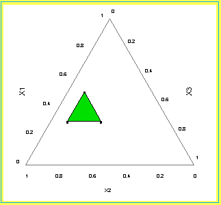
The feasible mixture space is shown in the figure below. Note that the existence of lower bounds does not affect the shape of the mixture region, it is still a simplex region. In general, this will always be the case if only lower bounds are imposed on any of the component proportions.

Diagram showing the feasible mixture space

FIGURE 5.12: The Feasible Mixture Space (Shaded Region) for Three Components with Lower Bounds

A simple transformation helps in design construction and analysis

Since the new region of the experiment is still a simplex, it is possible to define a new set of components that take on the values from 0 to 1 over the feasible region. This will make the design construction and the model fitting easier over the constrained region of interest. These new components ( \( x_{i}^{\star} \) ) are called pseudo components and are defined using the following formula

Formula for pseudo components

\[ x_{i}^{\star} = \frac{x_{i} - L_{i}} {1 - L} \]

with

\[ L = \sum_{i=1}^{q}{L_{i}} < 1 \]

denoting the sum of all the lower bounds.

Computation of the pseudo components for the example

In the three component example above, the pseudo components are

\( x_{1}^{\star} = \frac{x_{1} - 0.3}{0.2} \hspace{.3in} x_{2}^{\star} = \frac{x_{2} - 0.4}{0.2} \hspace{.3in} x_{3}^{\star} = \frac{x_{3} - 0.1}{0.2} \hspace{.3in} \)

Constructing the design in the pseudo components

Constructing a design in the pseudo components is accomplished by specifying the design points in terms of the and then converting them to the original component settings using

x_i = L_i + (1 - L)\( x_{i}^{\star} \)

Select appropriate design

In terms of the pseudo components, the experimenter has the choice of selecting a Simplex-Lattice or a Simplex-Centroid design, depending on the objectives of the experiment.

Simplex-centroid design example (after transformation)

Suppose, we decided to use a Simplex-centroid design for the three-component experiment. The table below shows the design points in the pseudo components, along with the corresponding setting for the original components.

Table showing the design points in both the pseudo components and the original components

TABLE 5.5: Pseudo Component Settings and Original Component Settings, Three-Component Simplex-Centroid Design

Pseudo Components				Original Components
X1	X2	X3		\( x_{1}^{\star} \)	\( x_{2}^{\star} \)	\( x_{3}^{\star} \)
1	0	0		0.5	0.4	0.1
0	1	0		0.3	0.6	0.1
0	0	1		0.3	0.4	0.3
0.5	0.5	0		0.4	0.5	0.1
0.5	0	0.5		0.4	0.4	0.2
0	0.5	0.5		0.3	0.5	0.2
0.3333	0.3333	0.3333		0.3667	0.4667	0.1666

Use of pseudo components (after transformation) is recommended

It is recommended that the pseudo components be used to fit the mixture model. This is due to the fact that the constrained design space will usually have relatively high levels of multicollinearity among the predictors. Once the final predictive model for the pseudo components has been determined, the equation in terms of the original components can be determined by substituting the relationship between x_i and \( x_{i}^{\star} \).

D-optimal designs can also be used

Computer-aided designs (D-optimal, for example) can be used to select points for a mixture design in a constrained region. See Myers and Montgomery (1995) for more details on using D-optimal designs in mixture experiments.

Extreme vertice designs are another option

Note: There are other mixture designs that cover only a sub-portion or smaller space within the simplex. These types of mixture designs (not covered here) are referred to as extreme vertices designs. (See chapter 11 of Myers and Montgomery (1995) or Cornell (1990).