SED navigation bar go to SED home page go to Dataplot home page go to NIST home page SED Home Page SED Staff SED Projects SED Products and Publications Search SED Pages
Dataplot Vol 1 Vol 2

CHI SQUARE GOODNESS OF FIT TEST

Name:
    ... CHI SQUARE GOODNESS OF FIT TEST

    NOTE: This command has been replaced with the unified GOODNESS OF FIT command.

Type:
    Analysis Command
Purpose:
    Perform a chi-square goodness of fit test that a set of data come from a hypothesized distributuion. Dataplot currently supports the chi-square goodness of fit test for 70+ distributions.
Description:
    The basic idea behind the chi-square goodness of fit test is to divide the range of the data into a number of intervals. Then the number of points that fall into each interval is compared to expected number of points for that interval if the data in fact come from the hypothesized distribution. More formally, the chi-square goodness of fit test statistic can be defined as follows.

    H0: The data follow the specified distribution.
    Ha: The data do not follow the specified distribution.
    Test Statistic: For the chi-square goodness of fit, the data is divided into k bins and the test statistic is defined as

      Chi-Square = SUM(O(i) - E(i))**2/E(i) where the
 summation is for bin 1 to k, O(i) is the observed frequency for bin i,
 and E(i) is the expected frequency for bin i

    where Oi is the observed frequency for bin i and Ei is the expected frequency for bin i. The expected frequency is calculated by

      E(i) = F(Y(u)) - F(Y(l))

    where F is the cumulative distribution function for the distribution being tested, Yu is the upper limit for class i, and Yl is the lower limit for class i.

    This test is sensitive to the choice of bins. There is no optimal choice for the bin width (since the optimal bin width depends on the distribution). Most reasonable choices should produce similar, but not identical, results. Dataplot uses 0.3*s, where s is the sample standard deviation, for the class width. The lower and upper bins are at the sample mean plus and minus 6.0*s respectively. For the chi-square approximation to be valid, the expected frequency should be at least 5. This test is not valid for small samples, and if some of the counts are less than five, you may need to combine some bins in the tails.

    Significance Level: alpha
    Critical Region: The test statistic follows, approximately, a chi-square distribution with (k - c) degrees of freedom where k is the number of non-empty cells and c = the number of parameters (including location and scale parameters and shape parameters) for the distribution + 1. For example, for a 3-parameter Weibull distribution, c = 4.

    Therefore, the hypothesis that the distribution is from the specified distribution is rejected if

      Chi-Square > CHSPPF(1-alpha,k-c)

    where CHSPPF 
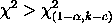
is the chi-square percent point function 
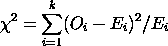
with k - c degrees of freedom and a significance level of alpha.

    The primary advantage of the chi square goodnes of fit test is that it is quite general. It can be applied for any distribution, either discrete or continuous, for which the cumulative distribution function can be computed. Dataplot supports the chi-square goodness of fit test for all distributions for which it supports a CDF function.

    There are two primary disadvantages:

    1. The test is sensitive to how the binning of the data is performed.
    2. It requires sufficient sample size so that the minimum expected frequency is five.

    In order to apply the chi-square goodness of fit test, any shape parameters must be specified. For example,

      LET GAMMA = 5.3
      WEIBULL CHI-SQUARE GOODNESS OF FIT TEST Y

    The name of the distributional parameter for families is given in the list below.

    Location and scale parameters can be specified generically with the following commands:

      LET CHSLOC = <value>
      LET CHSSCALE = <value>

    The location and scale parameters default to 1 if not specified.

    Dataplot supports the chi-square goodness of fit test for either binned or unbinned data.

    For unbinned data, Dataplot automatically generates binned data using the same rule as for histograms. That is, the class width is 0.3*s where s is the sample standard devition. The upper and lower limits are the mean plus or minus 6 times the sample standard deviation (any zero frequency bins in the tails are omitted). As with the HISTOGRAM command, you can override these defaults using the CLASS WIDTH, CLASS UPPER, and CLASS LOWER commands.

    Pre-binned data can be specicied in two ways. If your bins are of equal size, then you specify a single X variable that contains the mid-points of the bins. If your bins may be of unequal size, then two X variables are given. The first contains the lower limit of each bin and the second contains the upper limit of each bin. Unequal bin sizes usually result from combining classes with small (less than 5) expected frequency.

Syntax 1:
    <dist> CHI-SQUARE GOODNESS OF FIT TEST <y> <SUBSET/EXCEPT/FOR/qualification>
    where <y> is a response variable;
              <dist> is one of the following distributions:
      1. UNIFORM
      2. SEMI-CIRCULAR
      3. TRIANGULAR
      4. NORMAL
      5. LOGISTIC
      6. DOUBLE EXPONENTIAL
      7. CAUCHY
      8. TUKEY LAMBDA (LAMBDA)
      9. LOGNORMAL (SD, optional, defaults to 1)
      10. HALFNORMAL
      11. T (NU)
      12. CHI-SQUARED (NU)
      13. F (NU1, NU2)
      14. EXPONENTIAL
      15. GAMMA (GAMMA)
      16. BETA (ALPHA, BETA)
      17. WEIBULL (GAMMA)
      18. EXTREME VALUE TYPE 1
      19. EXTREME VALUE TYPE 2 (GAMMA)
      20. PARETO (GAMMA)
      21. BINOMIAL (N, P)
      22. GEOMETRIC (P)
      23. POISSON (LAMBDA)
      24. NEGATIVE BINOMIAL (N, K, P)
      25. WALD (GAMMA)
      26. INVERSE GAUSSIAN (GAMMA)
      27. RIG (GAMMA)
      28. FL (GAMMA)
      29. DISCRETE UNIFORM (N)
      30. NONCENTRAL BETA (ALPHA, BETA, LAMBDA)
      31. NONCENTRAL CHISQUARE (NU, LAMBDA)
      32. NONCENTRAL F (NU1, NU2, LAMBDA)
      33. DOUBLY NONCENTRAL F (NU1, NU2, LAMBDA1, LAMBDA2)
      34. NONCENTRAL T (NU, LAMBDA)
      35. DOUBLY NONCENTRAL T (NU, LAMBDA1, LAMBDA2)
      36. HYPERGEOMETRIC (K, N, M)
      37. VON-MISES (B)
      38. POWER-NORMAL (P, SD)
      39. POWER-LOGNORMAL (P, SD)
      40. COSINE
      41. ALPHA (ALPHA, BETA)
      42. POWER FUNCTION (C)
      43. CHI (NU)
      44. LOGARITHMIC SERIES (THETA)
      45. LOG LOGISTIC (DELTA)
      46. GENERALIZED GAMMA (GAMMA, C)
      47. WARING (A, C, if C omitted, have YULE distribution)
      48. ANGLIT
      49. ARCSIN
      50. HYPERBOLIC SECANT
      51. HALF CAUCHY
      52. FOLDED NORMAL (M, SD)
      53. TRUNCATED NORMAL (A, B, M, SD)
      54. TRUNCATED EXPONENTIAL (X0, M, SD)
      55. DOUBLE WEIBULL (GAMMA)
      56. LOG GAMMA (GAMMA)
      57. GENERALIZED EXTREME VALUE (GAMMA)
      58. PARETO SECOND KIND (GAMMA)
      59. HALF LOGISTIC (GAMMA, optional)
      60. EXPONENTIATED WEIBULL (GAMMA, THETA)
      61. GOMPERTZ (C,B)
      62. WRAPPED CAUCHY (C)
      63. BETA BINOMIAL (ALPHA, BETA)
      64. BRADFORD (ALPHA, BETA)
      65. DOUBLE GAMMA (GAMMA)
      66. FOLDED CAUCHY (M, SD)
      67. GENERALIZED EXPONENTIAL (LAMBDA1, LAMBDA2, S)
      68. GENERALIZED LOGISTIC (ALPHA)
      69. MIELKE BETA-KAPPA (BETA, THETA, K)
      70. EXPONENTIAL POWER (ALPHA, BETA)
    and where the <SUBSET/EXCEPT/FOR qualification> is optional.

    This syntax is used for the case where you have unbinned data.

Syntax 2:
    <dist> CHI-SQUARE GOODNESS OF FIT TEST <y> <x> <SUBSET/EXCEPT/FOR/qualification>
    where <y> is a variable of pre-computed frequencies;
              <x> is a variable containing the mid-points of the bins;
              <dist> is as above;
    and where the <SUBSET/EXCEPT/FOR qualification> is optional.

    This syntax is used for the case where you have binned data with equal size bins.

Syntax 3:
    <dist> CHI-SQUARE GOODNESS OF FIT TEST <y> <x1> <x2> <SUBSET/EXCEPT/FOR/qualification>
    where <y> is a variable of pre-computed frequencies;
              <x1> is a variable containing the lower limits of the bins;
              <x2> is a variable containing the upper limits of the bins;
              <dist> is as above;
    and where the <SUBSET/EXCEPT/FOR qualification> is optional.

    This syntax is used for the case where you have binned data with unequal size bins.

Examples:
    NORMAL CHI-SQUARE GOODNESS OF FIT TEST Y
    NORMAL CHI-SQUARE GOODNESS OF FIT TEST Y SUBSET GROUP > 1
    CAUCHY CHI-SQUARE GOODNESS OF FIT TEST Y
    LOGNORMAL CHI-SQUARE GOODNESS OF FIT TEST X
    EXTREME VALUE TYPE 1 CHI-SQUARE GOODNESS OF FIT TEST X
    LET LAMBDA = 0.2
    TUKEY LAMBDA CHI-SQUARE GOODNESS OF FIT TEST X

    SET MINMAX = 1
    LET GAMMA = 2.0
    WEIBULL CHI-SQUARE GOODNESS OF FIT TEST X

    LET LAMBDA = 3
    POISSON CHI-SQUARE GOODNESS OF FIT TEST X

    NORMAL CHI-SQUARE GOODNESS OF FIT TEST Y X
    NORMAL CHI-SQUARE GOODNESS OF FIT TEST Y X1 X2

Note:
    There are several approaches for estimating the parameters of a distribution before applying the goodness of fit test. PPCC plots combined with probability plots are an effective graphical approach if there are zero or one shape parameters. Maximum likelihood estimation is available for several distributions. Least squares estimation can be applied for distributions for which maximum likelihood estimation is not available.
Note:
    The bin number, bin mid-point, observed frequency, and expected frequency are written to the file DPST1F.DAT (dpst1f.dat under Unix) in the current directory.
Note:
    The CHI-SQUARE GOODNESS OF FIT command automatically saves the following parameters. STATVAL - value of the chi-square goodness of fit statistic STATNU - degrees of freedom for the chi-square goodness of fit test STATCDF - cdf value for the chi-square goodness of fit test statistic CUTUPP90 - 90% critical value (alpha = 0.10) for the chi-square goodness of fit test statistic CUTUPP95 - 95% critical value (alpha = 0.05) for the chi-square goodness of fit test statistic CUTUPP99 - 99% critical value (alpha = 0.01) for the chi-square goodness of fit test statistic These parameters can be used in subsequent analysis.
Default:
    Location and scale parameters default to zero and one. Shape parameters must be explicitly specified. There is no default distribution.
Synonyms:
    EV2 and FRECHET are synonyms for EXTREME VALUE TYPE 2.
    EV1 and GUMBEL are synonyms for EXTREME VALUE TYPE 1.
    FATIGUE LIFE is a synonym for FL.
    RECIPROCAL INVERSE GAUSSIAN is a synonym for RIG.
    IG is a synonym for INVERSE GAUSSIAN.

    The word TEST is optional.

    CHI-SQUARE, CHISQUARE, and CHI SQUARE can all be used.

Related Commands:
    ANDERSON-DARLING TEST = Perform Anderson-Darling test for goodness of fit.
    KOLMOGOROV-SMIRNOV TEST = Perform Kolmogorov-Smirnov test for goodness of fit.
    WILK-SHAPIRO TEST = Perform Wilk-Shapiro test for normality.
    MAXIMUM LIKELIHOOD = Perform maximum likelihood estimation for several distributions.
    FIT = Perform least squares fitting.
    PROBABILITY PLOT = Generates a probability plot.
    HISTOGRAM = Generates a histogram.
    PPCC PLOT = Generates probability plot correlation coefficient plot.
    CLASS WIDTH = Specify the class width.
    CLASS UPPER = Specify the upper limit for classes.
    CLASS LOWER = Specify the lower limit for classes.
Reference:
    "Statistical Methods", Eight Edition, Snedecor and Cochran, Iowa State, 1989, pp. 76-79.
Applications:
    Distributional Analysis
Implementation Date:
    1998/12
Program:
    skip 25
    read zarr13.dat y
    .
    let m = mean y
    let s = standard deviation y
    let chsloc = m
    let chsscale = s
    normal chi-square goodness of fit test y

    The following output is generated.

          ************************************************
          **  normal chi-square goodness of fit test y  **
          ************************************************
     
     
                      CHI-SQUARED GOODNESS OF FIT TEST
     
    NULL HYPOTHESIS H0:      DISTRIBUTION FITS THE DATA
    ALTERNATE HYPOTHESIS HA: DISTRIBUTION DOES NOT FIT THE DATA
    DISTRIBUTION:            NORMAL
     
    SAMPLE:
       NUMBER OF OBSERVATIONS      =      195
       NUMBER OF NON-EMPTY CELLS   =       20
       NUMBER OF PARAMETERS USED   =        2
     
    TEST:
    CHI-SQUARED TEST STATISTIC     =    5.506083
       DEGREES OF FREEDOM          =       17
       CHI-SQUARED CDF VALUE       =    0.004063
     
       ALPHA LEVEL         CUTOFF              CONCLUSION
               10%       24.76903               ACCEPT H0
                5%       27.58711               ACCEPT H0
                1%       33.40867               ACCEPT H0
     
          CELL NUMBER, BIN MIDPOINT, OBSERVED FREQUENCY, AND
          EXPECTED FRQUENCY
          WRITTEN TO FILE DPST1F.DAT
        
Date created: 06/05/2001
Last updated: 12/11/2023

Please email comments on this WWW page to alan.heckert@nist.gov.