HOTELLING CONTROL CHART

HOTELLING CONTROL CHART

Graphics Command

Generates a multivariate Hotelling control chart.

An \( \bar{X} \) control chart is a data analysis analysis technique for determining if a univariate measurement process has gone out of statistical control. In many cases, there will be more than one measurement process to monitor. One approach to multivariate measurement processes, say with k measurements, is simply to generate the k individual \( \bar{X} \) charts. The drawback to this approach is that it does not account for correlation between the measurement processes.

The Hotelling control chart is a multivariate extension of the \( \bar{X} \) chart that does take the correlation into account. Note that the following cases need to be distinguished:

1. The data can consist of subgroups or individual observations.

2. There are two phases for control charts. Phase I is the startup case. That is, we use the data collected in the phase I startup to establish the control limits. For phase II, a distinction is made between "historical" data and "future" data. Historical data, collected in phase I, is used to generate the control limits for the future (i.e., phase II) data.

   The distinction between phase I and phase II exists for univariate \( \bar{X} \) charts. However, this distinction is typically ignored in practice. It should not be ignored for multivariate Hotelling charts.

Combining the above results in the following four cases:

1. Phase I with subgroups

   Given p response variables, the phase I subgroup Hotelling control chart plots the following quantity:

   \( T^{2} = n(\bar{x} - \bar{\bar{x}}_{0})'s^{-1}(\bar{x} - \bar{\bar{x}}_{0}) \)

   with n denoting the size of the subgroup, is \( \bar{\bar{X}} \) the vector of the p sample means of the subgroup means, \( \bar{X} \) is the vector of the p sample subgroup means, and \( S_{p}^{-1} \) is the inverse of the pooled covariance matrix.

   Note that this is essentially a 1-sample Hotelling test for whether the means for a given sbgroup are equal to the overall sample means.

   The Hotelling control chart then plots the sample T² test statistic on the vertical axis and the subgroup identifier on the horizontal axis.

   The upper control limit (there is no lower control limit) for this case is

   \( UCL = \frac{knp - kn - np + p}{kn - k -p +1} F_{\alpha;p,kn-k-p+1} \)

   with n denoting the subgroup size, k the number of subgroups, and p the number of variables. The value of \( \alpha \) for the F test is chosen so that \( \alpha \)/(2p) = 0.00135. This corresponds to the 3-sigma value for the univariate control chart.

2. Phase II with subgroups

   For phase II, the \( \bar{\bar{X}} \) and \( S_{p}^{-1} \) are computed from the historical data only. For the historical data, if any points were outside the control limits and assignable causes were determined, these observations are omitted from the computation of \( \bar{\bar{X}} \) and \( S_{p}^{-1} \) (note that all observations in the subgroup are omitted). The number of discarded groups will be denoted by na (na may be zero).

   The T² value is computed for future points as in phase I, except that \( \bar{\bar{X}} \) and \( S_{p}^{-1} \) are based on the non-discarded groups in the historical data only.

   The control limits for this case are

   \( UCL = \frac{p(k-na+1)(n-1)}{(k-na)n-k+na-p+1} F_{\alpha;p,(k-na)n-k+na-p+1} \)

3. Phase I with individual observations

   When there are m observations with no subgroups, the plotted statistic is

   \( Q_{j} = (x - \bar{x}_{m})'s_{m}^{-1}(x - \bar{x}_{m}) \)

   with \( \bar{x}_{m} \) denoting the vector of p means for all the data and \( S_{m}^{-1} \) denoting the covariance matrix of all m observations.

   The control limits are

   \( UCL = \frac{(m-1)^2}{m} B_{1-\alpha/2;p/2,(m-p-1)/2} \)

   \( LCL = \frac{(m-1)^2}{m} B_{\alpha/2;p/2,(m-p-1)/2} \)

   where \( B(\cdot) \) is the percent point function of the Beta distribution and \( \alpha \) is the significance level (typically set to 0.05 or 0.01).

   It is primarily the upper control limit that is of interest.

4. Phase II with individual observations

   The phase II Q_j is computed as for the phase I Q_j except that \( \bar{x}_{m} \) and \( S_{m}^{-1} \) are computed from the historical data only. Again, any historical data that are plotted outside the control limits and had an assignable cause determined are discarded. The control limits are

   \( UCL = \frac{p(m+1)(m-1)}{m^2 - mp} F_{1-\alpha/2;p,m-p} \)

   \( LCL = \frac{p(m+1)(m-1)}{m^2 - mp} F_{\alpha/2;p,m-p} \)

   It is primarily the upper control limit that is of interest.

For phase II control charts, Dataplot uses an extra variable, called the history variable, to distinguish between historical and future data. Specifically,

-1	= the corresponding observation is a discarded historical value
0	= the corresponding observation is a historical value
1	= the corresponding observation is a future value

For subgroup data, if any observation in the group is denoted as a historical observation, all observations in that group are considered historical. Likewise, if any observation in the subgroup is marked as discarded, the entire subgroup is discarded.

You can set your own control limits by entering the commands:

LET USL = <value>
LET LSL = <value>

You can control the appearance of this chart by setting the switches for the LINE, CHARACTER, SPIKE, and BAR commands appropriately. Specifically,

1. Phase I, subgroups

   Trace 1	= T2 values
   Trace 2	= Dataplot calculated upper control limit
   Trace 3	= User specified upper control limit

2. Phase II, subgroups

   Trace 1	= T2 values for historical data
   Trace 2	= T2 values for future data
   Trace 3	= Dataplot calculated upper control limit
   Trace 4	= User specified upper control limit

3. Phase I, individual

   Trace 1	- Qj values
   Trace 2	= Dataplot calculated upper control limit
   Trace 3	= Dataplot calculated lower control limit
   Trace 4	= User specified upper control limit
   Trace 5	= User specified lower control limit

4. Phase II, individual

   Trace 1	- Qj values, historical
   Trace 2	- Qj values, future
   Trace 3	= Dataplot calculated upper control limit
   Trace 4	= Dataplot calculated lower control limit
   Trace 5	= User specified upper control limit
   Trace 6	= User specified lower control limit

The setting of the lines and characters is demonstrated in the example programs below.

For a more extensive discussion of multivariate control charts, see Ryan (2000), Montgomery (2001), or the NIST/Sematech e-Handbook of Statistical Methods.

PHASE I HOTELLING CONTROL CHART <y1> <y2> ... <yk> <group>
                        <SUBSET/EXCEPT/FOR qualification>
where <y1> <y2> ... <yk> is a list of response variables;
          <group> is an independent variable containing the sub-group identifications;
and where the <SUBSET/EXCEPT/FOR qualification> is optional.

PHASE II HOTELLING CONTROL CHART <y1> <y2> ... <yk> <group> <hist>
                        <SUBSET/EXCEPT/FOR qualification>
where <y1> <y2> ... <yk> is a list of response variables;
          <group> is an independent variable containing the sub-group identifications;
          <hist> is an independent variable that identifies observations as historical or future;
and where the <SUBSET/EXCEPT/FOR qualification> is optional.

PHASE I HOTELLING INDIVIDUAL CONTROL CHART <y1> <y2> ... <yk>
                        <SUBSET/EXCEPT/FOR qualification>
where <y1> <y2> ... <yk> is a list of response variables;
and where the <SUBSET/EXCEPT/FOR qualification> is optional.

PHASE II HOTELLING INDIVIDUAL CONTROL CHART <y1> <y2> ... <yk>
                        <SUBSET/EXCEPT/FOR qualification>
where <y1> <y2> ... <yk> is a list of response variables;
          <hist> is an independent variable that identifies observations as historical or future;
and where the <SUBSET/EXCEPT/FOR qualification> is optional.

HOTELLING PHASE I CONTROL CHART Y1 Y2 Y3 GROUP
HOTELLING PHASE II CONTROL CHART Y1 Y2 Y3 GROUP HISTORY
HOTELLING PHASE I INDIVIDUAL CONTROL CHART Y1 Y2 Y3
HOTELLING PHASE II INDIVIDUAL CONTROL CHART Y1 Y2 Y3 HISTORY

For the individual Hotelling control charts, the desired significance level can be specified with the command
LET ALPHA = <value>

The most typical values for alpha are 0.05 and 0.01. The default is 0.05.

Some authors do not specify a lower control limit for the individual observations case. If this is your preference, set the line type for the lower control limit to BLANK and double the value of alpha (e.g., LET ALPHA = 0.10 to have an upper alpha value of 1 - .10/2 = 0.95).

The command HOTELLING CONTROL CHART will generate a PHASE I HOTELLING CONTROL CHART.

MULTIVARIATE is a synonym for HOTELLING
HOTELLING PHASE xx is a synonym for PHASE xx HOTELLING
PHASE 1 and PHASE ONE are synonyms for PHASE I
PHASE 2 and PHASE TWO are synonyms for PHASE II

XBAR CONTROL CHART	= Generates a mean control chart.
RANGE CONTROL CHART	= Generates a mean control chart.
S CONTROL CHART	= Generates a sd control chart.
CUSUM CONTROL CHART	= Generates a mean cusum control chart.
EWMA CONTROL CHART	= Generates a ewma control chart.
MOVING AVERAGE CHART	= Generates a moving average control chart.
MOVING RANGE CHART	= Generates a moving range control chart.
MOVING SD CHART	= Generates a moving sd control chart.
C CHART	= Generates a C control chart.
U CHART	= Generates a U control chart.
P CHART	= Generates a P control chart.
NP CHART	= Generates an Np control chart.

"Statistical Methods For Quality Improvement", 2nd. Ed., Thomas Ryan, John Wiley and Sons, 2000, Chapter 9.

"Introduction To Statistical Quality Control", 4th. ed., Douglass Montgomery, John Wiley and Sons, 2001, Chapter 10.

"Multivariate Control Charts for Individual Observations", Nola Tracy, John Young, and Robert Mason, Journal of Quality Technology, Vol. 24, No. 2, April 1992, 88-95.

"NIST/SEMATECH e-Handbook of Statistical Methods"

Quality Control

1998/9
2003/2: Implemented the four distinct cases (1998/9 implementation was for the phase I subgroup case only)

skip 25
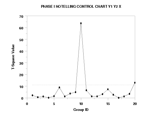
read t2cc.dat y1 y2 x
.
label case asis
line solid dot dot
character circle blank blank
character size 1.5
character fill on
title automatic
y1label T-Square Value
x1label Group ID
.
phase I hotelling control chart y1 y2 x
    

skip 25
read t2cc.dat y1 y2 x
let n = size x
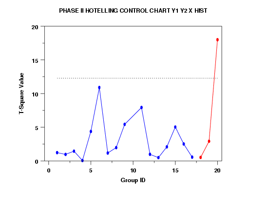
let hist = 0 for i = 1 1 n
let hist = -1 subset x = 10
let hist = 1 subset x > 17
.
label case asis
line solid solid dot dot
line color blue red black black
character circle circle blank blank
character color blue red 
character size 1.5 1.5
character fill on on
title automatic
y1label T-Square Value
x1label Group ID
xtic offset 0.5 0.5
.
phase II hotelling control chart y1 y2 x hist
    

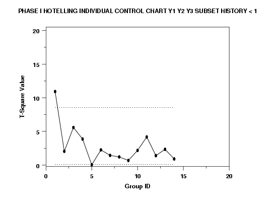
.  Following data is from the Tracy, Young, and Mason article
read y1 y2 y3 history
14.92    85.77   42.26    -1
16.90    83.77   43.44     0
17.38    84.46   42.74     0
16.90    86.27   43.60     0
16.92    85.23   43.18     0
16.71    83.81   43.72     0
17.07    86.08   43.33     0
16.93    85.85   43.41     0
16.71    85.73   43.28     0
16.88    86.27   42.59     0
16.73    83.46   44.00     0
17.07    85.81   42.78     0
17.60    85.92   43.11     0
16.90    84.23   43.48     0
17.08    84.08   43.81     1
end of data
.
label case asis
line solid dot dot
character circle blank blank
character size 1.5
character fill on
title automatic
y1label T-Square Value
x1label Group ID
ytic offset 0.2 0.5
.
let alpha = .01
.
phase I hotelling individual control chart y1 y2 y3 subset history < 1
.
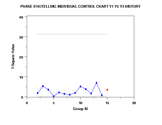
line solid solid dot dot
line color blue red
character color blue red
character circle circle blank blank
character size 1.5 all
character fill on on
phase II hotelling individual control chart y1 y2 y3 history