SINGLE SAMPLE ACCEPTANCE PLAN

SINGLE SAMPLE ACCEPTANCE PLAN

Analysis Command

Generates a single sample acceptance plan.

A lot acceptance sampling plan is a sampling scheme and a set of rules for making decisions. The decision, based on counting the number of defectives in a sample, can be to accept the lot, reject the lot, or to take another sample.

For a single sampling plan, one sample of items is selected at random from a lot and the disposition of the lot is determined from the resulting information. These plans are also denoted as (n,c) plans since there are n observations and the lot is rejected if there are more than c defectives.

Single sample acceptance plans are the most common and easiest plans to use. However, they are not the most efficient in terms of the average number of samples needed.

The input to this command is the following four parameters:

1. P1 = the acceptable quality level (AQL). The AQL is the a proportion defective that is the base line requirement for the quality of the producer's product. The producer would like to design a sampling plan such that there is a high probability of accepting a lot that has a defect level less than or equal to the AQL. In Dataplot, this value should be entered as a proportion (i.e., a value between 0 and 1.0).

2. P2 = the lot tolerance percent defective (LTPD). The LTPD is a designated high defect level that would be unacceptable to the consumer. The consumer would like the sampling plan to have a low probability of accepting a lot with a defect level as high as the LTPD. In Dataplot, this value should be entered as a proportion (i.e., a value between 0 and 1.0).

3. ALPHA = the Type I Error (Producers Risk). This is the probability, for a given (n,c) sampling plan, of rejecting a lot that has a defect level equal to the AQL. The producer suffers when this occurs because a lot with acceptable was rejected. Typical values for ALPHA range from 0.2 to 0.01.

4. BETA = the Type II Error (Consumers Risk). This is the probability, for a given (n,c) sampling plan, of accepting a lot with a defect level equal to the LTPD. The consumer suffers when this occurs because a lot with unacceptable quality was accepted. Typical values for BETA range from 0.2 to 0.01.

The output is the following two numbers:

1. N = the size sample to collect.
2. C = reject the lot if this number of defectives exceeded.

SINGLE SAMPLE ACCEPTANCE PLAN <p1> <p2> <alpha> <beta>
where <p1>is a number or parameter that specifies the AQL;
            <p2>is a number of parameter that specifies the LTPD;
            <alpha> is a number or parameter that is the producers risk;
and where <beta> is a number or parameter that is the consumers risk.

SINGLE SAMPLE ACCEPTANCE PLAN 0.98 0.05 0.01 0.10


LET P1 = 0.98
LET P2 = 0.05
LET ALPHA = 0.01
LET BETA = 0.10
SINGLE SAMPLE ACCEPTANCE PLAN P1 P2 ALPHA BETA

In addition to printing the values of N and C, Dataplot stores these values in the internal parameters SSN and SSNC. These parameters can be used in subsequent Dataplot analysis if needed.

Dataplot provides the following related macros:
• OC_SSB.DP - generate an Operating Characteristic (OC) curve assuming binomial probabilities. The OC curve is a plot of probability of acceptance versus percent defective.

• OC_SSA.DP - generate an Operating Characteristic (OC) curve assuming hypergeometric probabilities. The OC curve is a plot of probability of acceptance versus percent defective.

• AOQSS.DP - generate an Average Outgoing Quality (AOQ) curve. For non-destructive samples, rejected lots are often 100% inspected and defective units are replaced with good units. This means that the only defective units are those in lots that were accepted. The AOQ is the long term defect level for these combined lots. The AOQ curve is a plot of this AOQ versus percent defective.

• ATISS.DP - generate an Average Total Inspection (ATI) curve. The ATI curve is a plot of probability of acceptance versus lot fraction defective.

You can enter LIST where is the name of one of the macros above for details on how to use them.

None

None

CONTROL CHART	= Generate various types of control charts.
CP	= Compute a Cp capability index.
CUSUM ARL	= Generate a cusum average run length chart.

Douglas Montgomery (1981), "Introduction to Statistical Quality Control," John Wiley, 1991.

Quality Control

1999/3

 
LET P1 = 0.01
LET P2 = 0.05
LET ALPHA = 0.05
LET BETA = 0.10
SINGLE SAMPLE ACCEPTANCE PLAN P1 P2 ALPHA BETA
.
LET N = SSN
LET C = SSC
.
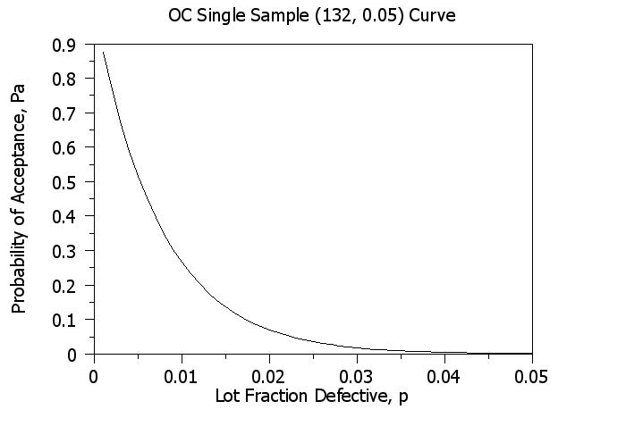
. Purpose--Generate an Operating Characteristic curve for a
.          single sample plan.  The OC is defined as:
.            BINCDF(c,p,n) versus p
.          where 
.            n      = sample size
.            c      = acceptance number for defectives
.            p      = desired binomial probabilities
.
LABEL CASE ASIS
TITLE CASE ASIS
Y1LABEL Probability of Acceptance, Pa
X1LABEL Lot Fraction Defective, p 
TITLE OC Single Sample (^SSN, ^SSC) Curve
.
PLOT BINCDF(SSC,P,SSN) FOR P = 0.001 0.001 0.05