SED navigation bar go to SED home page go to Dataplot home page go to NIST home page SED Home Page SED Staff SED Projects SED Products and Publications Search SED Pages
Dataplot Vol 2 Vol 1

BGEPDF

Name:
    BGEPDF (LET)
Type:
    Library Function
Purpose:
    Compute the beta-geometric probability mass function with shape parameters alpha and beta.
Description:
    If the probability of success parameter, p, of a geometric distribution has a Beta distribution with shape parameters alpha and beta, the resulting distribution is referred to as a beta-geometric distribution. For a standard geometric distribution, p is assumed to be fixed for successive trials. For the beta-geometric distribution, the value of p changes for each trial.

    The beta-geometric distribution has the following probability density function:

      P(x;alpha,beta) = B(alpha+1,x+beta-1)/B(alpha,beta)
  x = 1, 2, ...; alpha, beta > 0

    with alpha, beta, and B denoting the two shape parameters and the complete beta function, respectively. See the documentation for the BETA command for a description of the complete beta function.

Syntax:
    LET <y> = BGEPDF(<x>,<alpha>,<beta>)
                            <SUBSET/EXCEPT/FOR qualification>
    where <x> is a number, parameter, or variable containing non-negative integer values;
                <alpha> is a number, parameter, or variable that specifies the first shape parameter;
                <beta> is a number, parameter, or variable that specifies the second shape parameter;
                <y> is a variable or a parameter (depending on what <x> is) where the computed beta-geometric pdf value is stored;
    and where the <SUBSET/EXCEPT/FOR qualification> is optional.
Examples:
    LET A = BGEPDF(4,0.5,0.9)
    LET A = BGEPDF(X,2.1,4)
    PLOT BGEPDF(X,ALPHA,BETA) FOR X = 1 1 20
Note:
    Some sources shift this distribution to start at x = 0. In this case, the probability mass function is

      P(x;alpha,beta) = B(alpha+1,x+beta)/B(alpha,beta)
  x = 0, 1, 2, ...; alpha, beta > 0

    We will refer to the first parameterization as the unshifted parameterization and the second parameterization as the shifted parameterization.

    To specify the shifted parameterization (i.e., starting at x = 0), enter the command

      SET BETA GEOMETRIC DEFINITION SHIFTED

    To reset the unshifted parameterization (i.e., starting at x = 1), enter the command

      SET BETA GEOMETRIC DEFINITION UNSHIFTED

    This distribution is also sometimes given with alpha and beta reversed. In this case, the probability mass functions become

      P(x;alpha,beta) = B(alpha+1,x+beta-1)/B(alpha,beta)
x = 1, 2, ...; alpha, beta > 0

      and

      P(x;alpha,beta) = B(alpha+1,x+beta)/B(alpha,beta)
x = 0, 1, 2, ...; alpha, beta > 0

    To use this parameterization, simply interchange the order in which you give the alpha and beta arguments to the BGEPDF command.
Note:
    The beta-geometric as given above is derived as a beta mixture of geometric random variables.

    Irwin developed the Waring distribution based on the Waring expansion. The probability mass function for the Waring distribution is

      P(x;c,a) = (c-a)*(a+x-1)!*c!/[c*(a-1)!*(c+x)!]
  x = 0, 1, 2, ...; a > 0; c > a

    The Waring distribution can be computed with the shifted form of the beta-geometric distribution with the following change in parameters:

      beta = a
      alpha = c - a

    If a = 1, then the Waring distribution reduces to the Yule distribution.

    You can compute the Waring (and Yule) distributions using the BGEPDF routine with the above re-parameterization or you can use the WARPDF or YULPDF routines directly (enter HELP WARPDF or HELP YULPDF for details).

Note:
    For a number of commands utilizing the beta-geometric distribution, it is convenient to bin the data. There are two basic ways of binning the data.

    1. For some commands (histograms, maximum likelihood estimation), bins with equal size widths are required. This can be accomplished with the following commands:

        LET AMIN = MINIMUM Y
        LET AMAX = MAXIMUM Y
        LET AMIN2 = AMIN - 0.5
        LET AMAX2 = AMAX + 0.5
        CLASS MINIMUM AMIN2
        CLASS MAXIMUM AMAX2
        CLASS WIDTH 1
        LET Y2 X2 = BINNED

    2. For some commands, unequal width bins may be helpful. In particular, for the chi-square goodness of fit, it is typically recommended that the minimum class frequency be at least 5. In this case, it may be helpful to combine small frequencies in the tails. Unequal class width bins can be created with the commands

        LET MINSIZE = <value>
        LET Y3 XLOW XHIGH = INTEGER FREQUENCY TABLE Y

      If you already have equal width bins data, you can use the commands

        LET MINSIZE = <value>
        LET Y3 XLOW XHIGH = COMBINE FREQUENCY TABLE Y2 X2

      The MINSIZE parameter defines the minimum class frequency. The default value is 5.

Note:
    You can generate beta-geometric random numbers, probability plots, and chi-square goodness of fit tests with the following commands:

      LET ALPHA = <value>
      LET BETA = <value>
      LET Y = BETA GEOMETRIC RANDOM NUMBERS FOR I = 1 1 N

      BETA GEOMETRIC PROBABILITY PLOT Y
      BETA GEOMETRIC PROBABILITY PLOT Y2 X2
      BETA GEOMETRIC PROBABILITY PLOT Y3 XLOW XHIGH

      BETA GEOMETRIC CHI-SQUARE GOODNESS OF FIT Y
      BETA GEOMETRIC CHI-SQUARE GOODNESS OF FIT Y2 X2
      BETA GEOMETRIC CHI-SQUARE GOODNESS OF FIT Y3 XLOW XHIGH

    To obtain the first frequency and sample mean estimates and the maximum likelihood estimates of alpha and beta, enter the command

      BETA GEOMETRIC MAXIMUM LIKELIHOOD Y
      BETA GEOMETRIC MAXIMUM LIKELIHOOD Y2 X2

    The maximim likelihood estimates are computed using the parameterization

      pi = alpha/(alpha+beta)

      theta = 1/(alpha+beta)

    The estimates for alpha and beta can be expressed in terms of pi and theta as

      alphahat=muhat/thetahat

      betahat=(1-muhat)/thetahat

    The maximim likelihood estimates are the solutions of the equations

      (n/pi) - SUM[i=1 to n][{SUM[r=1 to x(i)-1][1/(1-pi+(r-1)*theta)]}] = 0

      SUM[i=1 to n][{SUM[r=1 to x(i)-1][(r-1)/(1-pi+(r-1)*theta)] - 
SUM[r=1 to x(i)][(r-1)/(1+(r-1)*theta)]}] = 0

    Dataplot prints the estimates for both parameterizations.

    You can generate estimates of alpha and beta based on the maximum ppcc value or the minimum chi-square goodness of fit with the commands

      LET ALPHA1 = <value>
      LET ALPHA2 = <value>
      LET BETA1 = <value>
      LET BETA2 = <value>
      BETA GEOMETRIC KS PLOT Y
      BETA GEOMETRIC KS PLOT Y2 X2
      BETA GEOMETRIC KS PLOT Y3 XLOW XHIGH
      BETA GEOMETRIC PPCC PLOT Y
      BETA GEOMETRIC PPCC PLOT Y2 X2
      BETA GEOMETRIC PPCC PLOT Y3 XLOW XHIGH

    The default values of alpha1 and alpha2 are 0.5 and 5, respectively. The default values for beta1 and beta2 are 0.5 and 5, respectively. Due to the discrete nature of the percent point function for discrete distributions, the ppcc plot will not be smooth. For that reason, if there is sufficient sample size the KS PLOT (i.e., the minimum chi-square value) is typically preferred. However, it may sometimes be useful to perform one iteration of the PPCC PLOT to obtain a rough idea of an appropriate neighborhood for the shape parameters since the minimum chi-square statistic can generate extremely large values for non-optimal values of the shape parameters. Also, since the data is integer values, one of the binned forms is preferred for these commands.

Default:
    None
Synonyms:
    None
Related Commands:
    BGECDF = Compute the beta-geometric cumulative distribution function.
    BGECDF Compute the beta-geometric cumulative distribution function.
    BETPDF = Compute the beta probability density function.
    GEOPDF = Compute the geometric probability mass function.
    WARPDF = Compute the Waring probability mass function.
    YULPDF = Compute the Yule probability mass function.
    BBNPDF = Compute the beta-binomial probability mass function.
    BNBPDF = Compute the beta-negative binomial (generalized Waring) probability mass function.
    INTEGER FREQUENCY TABLE = Generate a frequency table at integer values with unequal bins.
    COMBINE FREQUENCY TABLE = Convert an equal width frequency table to an unequal width frequency table.
    KS PLOT = Generate a minimum chi-square plot.
    MAXIMUM LIKELIHOOD = Perform maximum likelihood estimation for a distribution.
Reference:
    Ole Hesselager (1994), "A Recursive Procedure for Calculations of Some Compound Distributions", Astin Bulliten, Vol. 24, No. 1, pp. 19-32.

    Sudhir R. Paul (2004), "Applications of the Beta Distribution" in "Handbook of the Beta Distribution", edited by Gupta and Nadarajah, Marcel-Dekker, pp. 431-436.

    J. O. Irwin (1963), "The Place of Mathematics in Medical and Biological Statistics", Journal of the Royal Statistical Society, Series A, 126, pp. 1-44.

    Johnson, Kotz, and Kemp (1992), "Univariate Discrete Distributions", Second Edition, Wiley, chapter 6.

Applications:
    Distributional Modeling
Implementation Date:
    2006/7
Program 1:
     
    XLIMITS 0 50
    XTIC OFFSET 0.5 0.5
    LINE BLANK
    SPIKE ON
    SPIKE THICKNESS 0.3
    .
    TITLE CASE ASIS
    LABEL CASE ASIS
    X1LABEL Number of Successes
    Y1LABEL Probability Mass
    .
    MULTIPLOT 2 2
    MULTIPLOT CORNER COORDINATES 0 0 100 95
    MULTIPLOT SCALE FACTOR 2
    .
    TITLE Alpha = 0.5, Beta = 0.5
    PLOT BGEPDF(X,0.5,0.5) FOR X = 0 1 50
    .
    TITLE Alpha = 3, Beta = 0.5
    PLOT BGEPDF(X,3.0,0.5) FOR X = 0 1 50
    .
    TITLE Alpha = 0.5, Beta = 3
    PLOT BGEPDF(X,0.5,3.0) FOR X = 0 1 50
    .
    TITLE Alpha = 3, Beta = 3
    PLOT BGEPDF(X,3.0,3.0) FOR X = 0 1 50
    .
    END OF MULTIPLOT
    .
    CASE ASIS
    JUSTIFICATION CENTER
    MOVE 50 97
    TEXT Beta-Geometric Probability Mass Functions
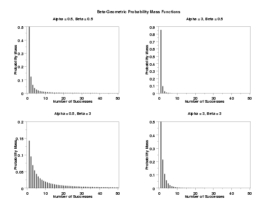
        
    plot generated by sample program

Program 2:
    let alpha = 1.3
    let beta = 3.1
    .
    let y = beta geometric random numbers for i = 1 1 200
    let y3 xlow xhigh = integer frequency table y
    class width 1
    let amin = minimum y
    let amin2 = amin - 0.5
    class lower amin2
    let amax = maximum y
    let amax2 = amax + 0.5
    class upper amax2
    let y2 x2 = binned y
    retain y2 x2 subset y2 > 0
    .
    beta geometric mle y2 x2
    let alpha = alphaml
    let beta  = betaml
    beta geometric chi-square goodness of fit test y3 xlow xhigh
    .
    title case asis
    title offset 2
    label case asis
    title Relative Histogram with Overlaid ML Fit PDF
    xlimits 0 100
    relative hist y2 x2
    limits freeze
    pre-erase off
    line color blue
    plot bgepdf(x,alpha,beta) for x = amin 1 amax
    limits
    pre-erase on
    line color black
    .
    title Probability Plot for ML Fit
    y1label Theoretical
    x1label Data
    x2label Alpha = ^alpha, Beta = ^beta
    char x
    line blank
    beta geometric probability plot y2 x2
    .
    title Minimum Chi-Square Plot
    y1label Chi-Square Value
    x1label Beta (Curves represent values of Alpha)
    x2label
    line solid all
    char blank all
    beta geometric ks plot y3 xlow xhigh
    justification center
    move 50 6
    text Alpha = ^shape1, Beta = ^shape2
    move 50 2
    text Minimum Chi-Square Value = ^minks
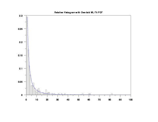
        
    plot generated by sample program

    plot generated by sample program

                 BETA-GEOMETRIC PARAMETER ESTIMATION:
      
     SUMMARY STATISTICS:
     NUMBER OF OBSERVATIONS                     =      200
     SAMPLE MEAN                                =    14.38000
     SAMPLE VARIANCE                            =    11258.67
     SAMPLE MINIMUM                             =    1.000000
     SAMPLE MAXIMUM                             =    1477.000
      
     FIRST FREQUENCY AND SAMPLE MEAN:
     ESTIMATE OF THETA                          =   0.2459736
     ESTIMATE OF PI                             =   0.2949999
     ESTIMATE OF ALPHA                          =    1.199316
     ESTIMATE OF BETA                           =    2.866162
      
     MAXIMUM LIKELIHOOD:
     ESTIMATE OF THETA                          =   0.2337158
     ESTIMATE OF PI                             =   0.2932754
     ESTIMATE OF ALPHA                          =    1.254837
     ESTIMATE OF BETA                           =    3.023863
     APPROXIMATE STANDARD ERROR OF PIHAT        =   0.1860668E-01
     APPROXIMATE STANDARD ERROR OF THETAHAT     =   0.4533415E-02
      
      
     THE COMPUTED VALUE OF THE CONSTANT ALPHA    =   0.1254837E+01
      
      
     THE COMPUTED VALUE OF THE CONSTANT BETA     =   0.3023863E+01
      
      
                       CHI-SQUARED GOODNESS-OF-FIT TEST
      
     NULL HYPOTHESIS H0:      DISTRIBUTION FITS THE DATA
     ALTERNATE HYPOTHESIS HA: DISTRIBUTION DOES NOT FIT THE DATA
     DISTRIBUTION:            BETA GEOMETRIC
      
     SAMPLE:
        NUMBER OF OBSERVATIONS      =      200
        NUMBER OF NON-EMPTY CELLS   =       15
        NUMBER OF PARAMETERS USED   =        2
      
     TEST:
     CHI-SQUARED TEST STATISTIC     =    12.16778
        DEGREES OF FREEDOM          =       12
        CHI-SQUARED CDF VALUE       =    0.567699
      
        ALPHA LEVEL         CUTOFF              CONCLUSION
                10%       18.54935               ACCEPT H0
                 5%       21.02607               ACCEPT H0
                 1%       26.21697               ACCEPT H0
        
    plot generated by sample program

Date created: 8/23/2006
Last updated: 8/23/2006
Please email comments on this WWW page to alan.heckert@nist.gov.