
|
BGEPPFName:
 and and
 . .
 and
and  ,
the resulting distribution is referred to as a beta-geometric
distribution. For a standard geometric distribution, p
is assumed to be fixed for successive trials. For the
beta-geometric distribution, the value of p changes
for each trial. ,
the resulting distribution is referred to as a beta-geometric
distribution. For a standard geometric distribution, p
is assumed to be fixed for successive trials. For the
beta-geometric distribution, the value of p changes
for each trial.
The beta-geometric distribution has the following probability density function:

with Dataplot computes the cumulative distribution function using a recurrence relation given by Hesselager. Hesselager gives the recurrence relation as:
![p(x;alpha,beta) = [(x+alpha-1)/(x+alpha+beta)]*p(x-1;alpha,beta)](eqns/bgecdf.gif)
Converting this to the parameterization above yields
![p(x;alpha,beta) = [(x+beta-2)/(x+alpha+beta-1)]*p(x-1;alpha,beta)](eqns/bgecdf2.gif)
Dataplot computes the percent point function by summing the cumulative distribution function until the specified probability is obtained.
<SUBSET/EXCEPT/FOR qualification> where <p> is a number, parameter, or variable in the interval (0,1); <alpha> is a number, parameter, or variable that specifies the first shape parameter; <beta> is a number, parameter, or variable that specifies the second shape parameter; <y> is a variable or a parameter (depending on what <p> is) where the computed beta-geometric ppf value is stored; and where the <SUBSET/EXCEPT/FOR qualification> is optional.
LET A = BGEPPF(P,2.1,4) PLOT BGEPPF(P,ALPHA,BETA) FOR P = 0 0.01 0.99

We will refer to the first parameterization as the unshifted parameterization and the second parameterization as the shifted parameterization. To specify the shifted parameterization (i.e., starting at x = 0), enter the command
To reset the unshifted parameterization (i.e., starting at x = 1), enter the command
This distribution is also sometimes given with

and
 and and
 arguments
to the BGEPPF command. arguments
to the BGEPPF command.
Irwin developed the Waring distribution based on the Waring expansion. The probability mass function for the Waring distribution is
![P(x;c,a) = (c-a)*(a+x-1)!*c!/[c*(a-1)!*(c+x)!]
x = 0, 1, 2, ...; a > 0; c > a](eqns/warpdf.gif)
The Waring distribution can be computed with the shifted form of the beta-geometric distribution with the following change in parameters:
 = a
= a
 = c - a
If a = 1, then the Waring distribution reduces to the Yule distribution. You can compute the Waring (and Yule) percent point functions using the BGEPPF routine with the above re-parameterization or you can use the WARPPF or YULPPF routines directly (enter HELP WARPDF or HELP YULPDF for details).
XLIMITS 0 1
XTIC OFFSET 0.5 0.5
.
TITLE CASE ASIS
LABEL CASE ASIS
Y1LABEL Number of Successes
X1LABEL Probability
TITLE DISPLACEMENT 2
Y1LABEL DISPLACEMENT 15
X1LABEL DISPLACEMENT 12
.
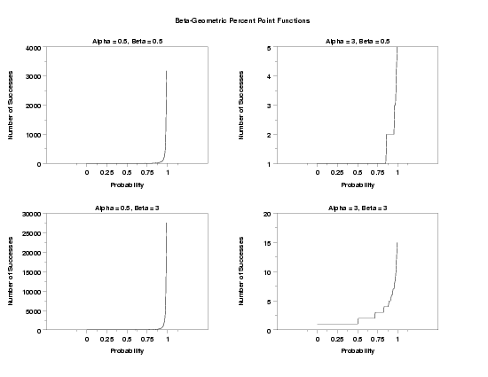
MULTIPLOT 2 2
MULTIPLOT CORNER COORDINATES 0 0 100 95
MULTIPLOT SCALE FACTOR 2
.
TITLE Alpha = 0.5, Beta = 0.5
PLOT BGEPPF(P,0.5,0.5) FOR P = 0  0.01  0.99
.
TITLE Alpha = 3, Beta = 0.5
PLOT BGEPPF(P,3.0,0.5) FOR P = 0  0.01  0.99
.
TITLE Alpha = 0.5, Beta = 3
PLOT BGEPPF(P,0.5,3.0) FOR P = 0  0.01  0.99
.
TITLE Alpha = 3, Beta = 3
PLOT BGEPPF(P,3.0,3.0) FOR P = 0  0.01  0.99
.
END OF MULTIPLOT
.
CASE ASIS
JUSTIFICATION CENTER
MOVE 50 97
TEXT Beta-Geometric Percent Point Functions

Date created: 8/23/2006 |