SED navigation bar go to SED home page go to Dataplot home page go to NIST home page SED Home Page SED Staff SED Projects SED Products and Publications Search SED Pages
Dataplot Vol 2 Vol 1

DIWPDF

Name:
    DIWPDF (LET)
Type:
    Library Function
Purpose:
    Compute the discrete Weibull probability mass function.
Description:
    The discrete Weibull distribution has the following probability mass function:

      p(x;q,beta) = (q)**(x**beta) - (q)**((x+1)**beta)
 x = 0, 1, 2, ...;
 0 < q < 1;  beta > 0

    with q and beta denoting the shape parameters.

    This distribution has application in reliability when the response of interest is a discrete variable.

Syntax:
    LET <y> = DIWPDF(<x>,<q>,<beta>)
                            <SUBSET/EXCEPT/FOR qualification>
    where <x> is a positive integer variable, number, or parameter;
                <q> is a number, parameter, or variable in the range (0,1) that specifies the first shape parameter;
                <beta> is a number, parameter, or variable that specifies the second shape parameter;
                <y> is a variable or a parameter (depending on what <x> is) where the computed discrete Weibull pdf value is stored;
    and where the <SUBSET/EXCEPT/FOR qualification> is optional.
Examples:
    LET A = DIWPDF(3,0.5,0.5)
    LET Y = DIWPDF(X,0.3,0.7)
    PLOT DIWPDF(X,0.6,0.4) FOR X = 1 1 20
Note:
    For a number of commands utilizing the discrete Weibull distribution, it is convenient to bin the data. There are two basic ways of binning the data.

    1. For some commands (histograms, maximum likelihood estimation), bins with equal size widths are required. This can be accomplished with the following commands:

        LET AMIN = MINIMUM Y
        LET AMAX = MAXIMUM Y
        LET AMIN2 = AMIN - 0.5
        LET AMAX2 = AMAX + 0.5
        CLASS MINIMUM AMIN2
        CLASS MAXIMUM AMAX2
        CLASS WIDTH 1
        LET Y2 X2 = BINNED

    2. For some commands, unequal width bins may be helpful. In particular, for the chi-square goodness of fit, it is typically recommended that the minimum class frequency be at least 5. In this case, it may be helpful to combine small frequencies in the tails. Unequal class width bins can be created with the commands

        LET MINSIZE = <value>
        LET Y3 XLOW XHIGH = INTEGER FREQUENCY TABLE Y

      If you already have equal width bins data, you can use the commands

        LET MINSIZE = <value>
        LET Y3 XLOW XHIGH = COMBINE FREQUENCY TABLE Y2 X2

      The MINSIZE parameter defines the minimum class frequency. The default value is 5.

Note:
    You can generate discrete Weibull random numbers, probability plots, and chi-square goodness of fit tests with the following commands:

      LET N = <N>
      LET Q = <value>
      LET BETA = <value>
      LET Y = DISCRETE WEIBULL ...
                  RANDOM NUMBERS FOR I = 1 1 N

      DISCRETE WEIBULL PROBABILITY PLOT Y
      DISCRETE WEIBULL PROBABILITY PLOT Y2 X2
      DISCRETE WEIBULL PROBABILITY PLOT ...
                  Y3 XLOW XHIGH

      DISCRETE WEIBULL CHI-SQUARE ...
                  GOODNESS OF FIT Y
      DISCRETE WEIBULL CHI-SQUARE ...
                  GOODNESS OF FIT Y2 X2
      DISCRETE WEIBULL CHI-SQUARE ...
                  GOODNESS OF FIT Y3 XLOW XHIGH

    You can generate estimates of q and beta based on the maximum ppcc value or the minimum chi-square goodness of fit with the commands

      LET Q1 = <value>
      LET Q2 = <value>
      LET BETA1 = <value>
      LET BETA2 = <value>
      DISCRETE WEIBULL KS PLOT Y
      DISCRETE WEIBULL KS PLOT Y2 X2
      DISCRETE WEIBULL KS PLOT Y3 XLOW XHIGH
      DISCRETE WEIBULL PPCC PLOT Y
      DISCRETE WEIBULL PPCC PLOT Y2 X2
      DISCRETE WEIBULL PPCC PLOT Y3 XLOW XHIGH

    The default values of Q1 and Q2 are 0.05 and 0.95, respectively. The default values for beta1 and beta2 are 0.1 and 3, respectively. Due to the discrete nature of the percent point function for discrete distributions, the ppcc plot will not be smooth. For that reason, if there is sufficient sample size the KS PLOT (i.e., the minimum chi-square value) is typically preferred. However, it may sometimes be useful to perform one iteration of the PPCC PLOT to obtain a rough idea of an appropriate neighborhood for the shape parameters since the minimum chi-square statistic can generate extremely large values for non-optimal values of the shape parameters. Also, since the data is integer values, one of the binned forms is preferred for these commands.

Default:
    None
Synonyms:
    None
Related Commands:
    DIWCDF = Compute the discrete Weibull cumulative distribution function.
    DIWCDF = Compute the discrete Weibull hazard function.
    DIWPPF = Compute the discrete Weibull percent point function.
    GLSPDF = Compute the generalized logarithmic series probability mass function.
    WEIPDF = Compute the Weibull probability density function.
    LGNPDF = Compute the lognormal probability density function.
    EXPPDF = Compute the exponential probability density function.
    POIPDF = Compute the Poisson probability mass function.
    BINPDF = Compute the binomial probability mass function.
    INTEGER FREQUENCY TABLE = Generate a frequency table at integer values with unequal bins.
    COMBINE FREQUENCY TABLE = Convert an equal width frequency table to an unequal width frequency table.
    KS PLOT = Generate a minimum chi-square plot.
    PPCC PLOT = Generate a ppcc plot.<
    PROBABILITY PLOT = Generate a probability plot.<
    MAXIMUM LIKELIHOOD = Perform maximum likelihood estimation for a distribution.
Reference:
    Johnson, Kemp, and Kotz (2005), "Univariate Discrete Distributions", Third Edition, Wiley, pp. 510-511.

    Nakagawa and Osaki (1975), "The Discrete Weibull Distribution", IEEE Transactions on Reliability, R-24, pp. 300-301.

Applications:
    Distributional Modeling
Implementation Date:
    2006/8
Program 1:
     
    title size 3
    tic label size 3
    label size 3
    legend size 3
    height 3
    x1label displacement 12
    y1label displacement 15
    .
    multiplot corner coordinates 0 0 100 95
    multiplot scale factor 2
    label case asis
    title case asis
    case asis
    tic offset units screen
    tic offset 3 3
    title displacement 2
    y1label Probability Mass
    x1label X
    .
    ylimits 0 0.2
    major ytic mark number 5
    minor ytic mark number 4
    xlimits 0 20
    line blank
    spike on
    .
    multiplot 2 2
    .
    title Q = 0.3, Beta = 0.3
    plot diwpdf(x,0.3,0.3) for x = 1 1 20
    .
    title Q = 0.5, Beta = 0.5
    plot diwpdf(x,0.5,0.5) for x = 1 1 20
    .
    title Q = 0.7, Beta = 0.7
    plot diwpdf(x,0.7,0.7) for x = 1 1 20
    .
    title Q = 0.9, Beta = 0.9
    plot diwpdf(x,0.9,0.9) for x = 1 1 20
    .
    end of multiplot
    .
    justification center
    move 50 97
    text Probability Mass Functions for Discrete Weibull
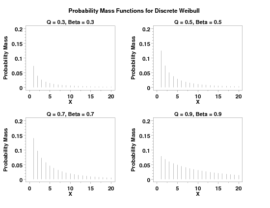
        
    plot generated by sample program

Program 2:
     
    let q = 0.4
    let beta = 0.5
    .
    let y = discrete weibull rand numbers for i = 1 1 500
    .
    let xmax = maximum y
    let xmax2 = xmax + 0.5
    let xmin = minimum y
    class lower -0.5
    class upper xmax2
    class width 1
    .
    let y2 x2 = binned y
    let y3 xlow xhigh = combine frequency table y2 x2
    .
    char blank
    line solid
    y1label Minimum Chi-Square
    x1label Beta (curves represent values of Q)
    discrete weibull ks plot y3 xlow xhigh
    justification center
    move 50 6
    text Minimum Chi-Square = ^minks
    .
    let q = shape1
    let beta = shape2
    char x
    line blank
    y1label Data
    x1label Theoretical
    discrete weibull prob plot y2 x2
    justification center
    move 50 6
    text PPCC = ^ppcc
    .
    line solid
    characters blank
    relative hist y2 x2
    limits freeze
    pre-erase off
    line color blue
    plot diwpdf(x,q,beta) for x = 0 1 xmax
    pre-erase on
    limits
    .
    discrete weibull chi-square goodness of fit y3 xlow xhigh
        
    The following graphs and output are generated.

    plot generated by sample program

    plot generated by sample program

    plot generated by sample program

                       CHI-SQUARED GOODNESS-OF-FIT TEST
      
     NULL HYPOTHESIS H0:      DISTRIBUTION FITS THE DATA
     ALTERNATE HYPOTHESIS HA: DISTRIBUTION DOES NOT FIT THE DATA
     DISTRIBUTION:            DISCRETE WEIBULL
      
     SAMPLE:
        NUMBER OF OBSERVATIONS      =      500
        NUMBER OF NON-EMPTY CELLS   =       13
        NUMBER OF PARAMETERS USED   =        2
      
     TEST:
     CHI-SQUARED TEST STATISTIC     =    7.480574
        DEGREES OF FREEDOM          =       10
        CHI-SQUARED CDF VALUE       =    0.320571
      
        ALPHA LEVEL         CUTOFF              CONCLUSION
                10%       15.98718               ACCEPT H0
                 5%       18.30704               ACCEPT H0
                 1%       23.20925               ACCEPT H0
        

Date created: 11/16/2006
Last updated: 11/16/2006
Please email comments on this WWW page to alan.heckert@nist.gov.