SED navigation bar go to SED home page go to Dataplot home page go to NIST home page SED Home Page SED Staff SED Projects SED Products and Publications Search SED Pages
Dataplot Vol 2 Vol 1

KUMPDF

Name:
    KUMPDF (LET)
Type:
    Library Function
Purpose:
    Compute the Kumaraswamy probability density function with shape parameters alpha and beta.
Description:
    The standard Kumaraswamy distribution has the following probability density function:

      f(x;alpha,beta) = alpha*beta*x**(alpha-1)*
(1-x**alpha)**(beta-1)     
0 <= x <= 1; alpha, beta > 0

    with alpha and beta denoting the shape parameters.

    This distribution can be extended with lower and upper bound parameters. If a and b denote the lower and upper bounds, respectively, then the location and scale parameters are:

      location = a
      scale = b - a

    The general form of the distribution can then be found by using the relation

      f(x;alpha,beta,a,b) = f((x-a)/(b-a);alpha,beta,0,1)/(b-a)

    This distribution has been proposed as a more tractable alternative to the beta distribution.

Syntax:
    LET <y> = KUMPDF(<x>,<alpha>,<beta>,<a>,<b>)
                            <SUBSET/EXCEPT/FOR qualification>
    where <x> is a number, parameter, or variable containing values in the interval (a,b);
                <y> is a variable or a parameter (depending on what <x> is) where the computed Kumaraswamy pdf value is stored;
                <alpha> is a positive number, parameter, or variable that specifies the first shape parameter;
                <beta> is a positive number, parameter, or variable that specifies the second shape parameter;
                <a> is a number, parameter, or variable that specifies the lower limit;
                <b> is a number, parameter, or variable that specifies the upper limit;
    and where the <SUBSET/EXCEPT/FOR qualification> is optional.

    If <a> and <b> are omitted, they default to 0 and 1, respectively.

Examples:
    LET A = KUMPDF(0.3,0.2,1.2)
    LET Y = KUMPDF(X,0.5,2)
    PLOT KUMPDF(X,2,3) FOR X = 0 0.01 1
Note:
    Kumaraswamy random numbers, probability plots, and goodness of fit tests can be generated with the commands:

      LET ALPHA = <value>
      LET BETA = <value>
      LET A = <value>
      LET B = <value>
      LET Y = KUMARASWAMY RANDOM NUMBERS FOR I = 1 1 N
      KUMARASWAMY PROBABILITY PLOT Y
      KUMARASWAMY PROBABILITY PLOT Y2 X2
      KUMARASWAMY PROBABILITY PLOT Y3 XLOW XHIGH
      KUMARASWAMY KOLMOGOROV SMIRNOV GOODNESS OF FIT Y
      KUMARASWAMY CHI-SQUARE GOODNESS OF FIT Y2 X2
      KUMARASWAMY CHI-SQUARE GOODNESS OF FIT Y3 XLOW XHIGH

    The following commands can be used to estimate the alpha and beta shape parameters for the Kumaraswamy distribution:

      LET ALPHA1 = <value>
      LET ALPHA2 = <value>
      LET BETA1 = <value>
      LET BETA2 = <value>
      KUMARASWAMY PPCC PLOT Y
      KUMARASWAMY PPCC PLOT Y2 X2
      KUMARASWAMY PPCC PLOT Y3 XLOW XHIGH
      KUMARASWAMY KS PLOT Y
      KUMARASWAMY KS PLOT Y2 X2
      KUMARASWAMY KS PLOT Y3 XLOW XHIGH

    The default values for ALPHA1 and ALPHA2 are 0.5 and 10. The default values for BETA1 and BETA2 are 0.5 and 10.

    The probability plot can then be used to estimate the lower and upper limits (lower limit = PPA0, upper limit = PPA0 + PPA1).

    The following options may be useful for these commands.

    1. Instead of generating the PPCC plot or KS plot on the original data, we can generate them on selected percentiles of the data. For example, if we have 1,000 points, we can choose to generate the plots on 100 evenly spaced percentiles with the command

        SET PPCC PLOT DATA POINTS 100

      This can be used to speed up the generation of the plot for larger data sets.

      Note that since the Kumaraswamy percent point function exists in closed form, this option is typically not needed.

    2. For the KS plot, we can fix the location and scale. This is equivalent to assuming that the lower and upper limits are known (e.g., we could use the data minimum and maximum as the lower and upper limit values). Given that the lower and upper limits are LOWLIM and UPPLIM, enter the commands

        LET KSLOC = LOWLIM
        LET KSSCALE = UPPLIM

      The PPCC plot is invariant to location and scale, so we cannot fix the lower and upper limits.

Default:
    None
Synonyms:
    None
Related Commands:
    KUMCDF = Compute the Kumaraswamy cumulative distribution function.
    KUMPPF = Compute the Kumaraswamy percent point function.
    RGTPDF = Compute the reflected generalized Topp and Leone probability density function.
    GTLPDF = Compute the generalized Topp and Leone probability density function.
    TOPPDF = Compute the Topp and Leone probability density function.
    TSPPDF = Compute the two-sided power probability density function.
    BETPDF = Compute the beta probability density function.
    TRIPDF = Compute the triangular probability density function.
    TRAPDF = Compute the trapezoid probability density function.
    UNIPDF = Compute the uniform probability density function.
    POWPDF = Compute the power probability density function.
    JSBPDF = Compute the Johnson SB probability density function.
Reference:
    Kumaraswamy (1980), "A Generalized Probability Density Function for Double-Bounded Random Processes", Journal of Hydrology, 46: 79-88.
Applications:
    Distributional Modeling
Implementation Date:
    2007/11
Program 1:
     
    CASE ASIS
    LABEL CASE ASIS
    TITLE CASE ASIS
    TITLE OFFSET 2
    .
    MULTIPLOT 3 3
    MULTIPLOT CORNER COORDINATES 0 0 100 95
    MULTIPLOT SCALE FACTOR 3
    .
    LET ALPHA = 2
    LET BETA  = 3
    TITLE Alpha = ^alpha, Beta = ^beta
    PLOT KUMPDF(X,ALPHA,BETA) FOR X = 0.01  0.01  0.99
    .
    LET ALPHA = 1.5
    LET BETA  = 6
    TITLE Alpha = ^alpha, Beta = ^beta
    PLOT KUMPDF(X,ALPHA,BETA) FOR X = 0.01  0.01  0.99
    .
    LET ALPHA = 1.5
    LET BETA  = 2
    TITLE Alpha = ^alpha, Beta = ^beta
    PLOT KUMPDF(X,ALPHA,BETA) FOR X = 0.01  0.01  0.99
    .
    LET ALPHA = 1.5
    LET BETA  = 1
    TITLE Alpha = ^alpha, Beta = ^beta
    PLOT KUMPDF(X,ALPHA,BETA) FOR X = 0.01  0.01  0.99
    .
    LET ALPHA = 0.5
    LET BETA  = 2
    TITLE Alpha = ^alpha, Beta = ^beta
    PLOT KUMPDF(X,ALPHA,BETA) FOR X = 0.01  0.01  0.99
    .
    LET ALPHA = 0.5
    LET BETA  = 1
    TITLE Alpha = ^alpha, Beta = ^beta
    PLOT KUMPDF(X,ALPHA,BETA) FOR X = 0.01  0.01  0.99
    .
    LET ALPHA = 0.5
    LET BETA  = 0.75
    TITLE Alpha = ^alpha, Beta = ^beta
    PLOT KUMPDF(X,ALPHA,BETA) FOR X = 0.01  0.01  0.99
    .
    LET ALPHA = 0.5
    LET BETA  = 0.25
    TITLE Alpha = ^alpha, Beta = ^beta
    PLOT KUMPDF(X,ALPHA,BETA) FOR X = 0.01  0.01  0.99
    .
    LET ALPHA = 1
    LET BETA  = 1
    TITLE Alpha = ^alpha, Beta = ^beta
    PLOT KUMPDF(X,ALPHA,BETA) FOR X = 0.01  0.01  0.99
    .
    END OF MULTIPLOT
    .
    JUSTIFICATION CENTER
    MOVE 50 97
    TEXT Kumaraswamy Probability Density Functions
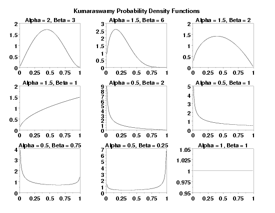
        
    plot generated by sample program

Program 2:
     
    let alpha = 1.2
    let beta = 2.6
    let alphasv = alpha
    let betasv = beta
    .
    let y = kuaraswamy rand numb for i = 1 1 200
    .
    kumaraswamy ppcc plot y
    justification center
    move 50 6
    let alpha = shape1
    let beta = shape2
    text Alpha = ^alpha, Beta = ^beta
    move 50 3
    text Alphasav = ^alphsav, Betasav = ^betasav
    .
    char x
    line blank
    kumaraswamy probability plot y
    move 50 6
    let lowlim = ppa0
    let upplim = ppa0 + ppa1
    text Lower Limit = ^lowlim, Upper Limit = ^upplim
    move 50 3
    text PPCC = ^ppcc
    char blank
    line solid
    let ksscale = upplim
    kumaraswamy kolm smir goodness of fit y
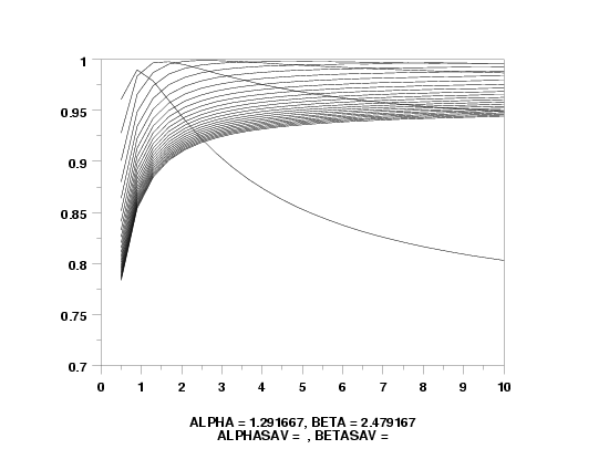
        
    plot generated by sample program

    plot generated by sample program

                       KOLMOGOROV-SMIRNOV GOODNESS-OF-FIT TEST
      
     NULL HYPOTHESIS H0:      DISTRIBUTION FITS THE DATA
     ALTERNATE HYPOTHESIS HA: DISTRIBUTION DOES NOT FIT THE DATA
     DISTRIBUTION:            KUMARASWAMY
        NUMBER OF OBSERVATIONS              =      200
      
     TEST:
     KOLMOGOROV-SMIRNOV TEST STATISTIC      =   0.3479910E-01
      
        ALPHA LEVEL         CUTOFF              CONCLUSION
                10%       0.086*              ACCEPT H0
                          0.085**
                 5%       0.096*              ACCEPT H0
                          0.095**
                 1%       0.115*              ACCEPT H0
                          0.114**
      
         *  - STANDARD LARGE SAMPLE APPROXIMATION  ( C/SQRT(N) )
        ** - MORE ACCURATE LARGE SAMPLE APPROXIMATION  ( C/SQRT(N + SQRT(N/10)) )
        

Date created: 11/27/2007
Last updated: 11/27/2007
Please email comments on this WWW page to alan.heckert@nist.gov.