LOSPDF

LOSPDF (LET)

Library Function

Compute the lost games probability mass function.

The formula for the lost games probability mass function is

with p and r denoting the shape parameters. The r parameter is restricted to non-negative integers.

This distribution is used to model the "gamblers ruin" problem. For this problem, p is the probability that the gambler loses one unit (1 - p is the probability that the gambler wins one unit). The value of r is the number of units the gambler starts with. The lost games distribution is then the distribution of the number of games lost until the gambler loses all of his fortune. This problem is referred to as the gambler's ruin since if the probability of winning is less than 0.5, the gambler will eventually lose all of his fortune with probability 1.

Although this distribution was developed to model gambling, Kemp and Kemp demonstrated its applicability to a number of other important applications. For example, Haight used it to model the queue with r initial customers, where new customers arrive according to a homogeneous Poisson process with shape parameter , and the service time follows an exponential distribution with shape parameter ( ≥ ). The p parameter in our formula can be expressed as

.

Note that Haight use the parameterization

Assuming a constant service time (rather than an exponential service time) results in the Borel-Tanner distribution.

LET <y> = LOSPDF(<x>,<p>,<r>)
                        <SUBSET/EXCEPT/FOR qualification>
where <x> is a positive integer variable, number, or parameter;
            <p> is a number or parameter in the range (0.5,1) that specifies the first shape parameter;
            <r> is a number or parameter denoting a positive integer that specifies the second shape parameter;
            <y> is a variable or a parameter where the computed lost games pdf value is stored;
and where the <SUBSET/EXCEPT/FOR qualification> is optional.

LET A = LOSPDF(3,0.7,3)
LET Y = LOSPDF(X1,0.7,2)
PLOT LOSPDF(X,0.6,5) FOR X = 5 1 50

For a number of commands utilizing the lost games distribution, it is convenient to bin the data. There are two basic ways of binning the data.
1. For some commands (histograms, maximum likelihood estimation), bins with equal size widths are required. This can be accomplished with the following commands:
   LET AMIN = MINIMUM Y
   LET AMAX = MAXIMUM Y
   LET AMIN2 = AMIN - 0.5
   LET AMAX2 = AMAX + 0.5
   CLASS MINIMUM AMIN2
   CLASS MAXIMUM AMAX2
   CLASS WIDTH 1
   LET Y2 X2 = BINNED
   

2. For some commands, unequal width bins may be helpful. In particular, for the chi-square goodness of fit, it is typically recommended that the minimum class frequency be at least 5. In this case, it may be helpful to combine small frequencies in the tails. Unequal class width bins can be created with the commands
   LET MINSIZE = <value>
   LET Y3 XLOW XHIGH = INTEGER FREQUENCY TABLE Y
   

   If you already have equal width bins data, you can use the commands

   LET MINSIZE = <value>
   LET Y3 XLOW XHIGH = COMBINE FREQUENCY TABLE Y2 X2
   

   The MINSIZE parameter defines the minimum class frequency. The default value is 5.

You can generate lost games random numbers, probability plots, and chi-square goodness of fit tests with the following commands:
LET N = VALUE
LET R = <value>
LET P = <value>
LET Y = LOST GAMES RANDOM NUMBERS FOR I = 1 1 N


LOST GAMES PROBABILITY PLOT Y
LOST GAMES PROBABILITY PLOT Y2 X2
LOST GAMES PROBABILITY PLOT Y3 XLOW XHIGH


LOST GAMES CHI-SQUARE GOODNESS OF FIT Y
LOST GAMES CHI-SQUARE GOODNESS OF FIT Y2 X2
LOST GAMES CHI-SQUARE GOODNESS OF FIT Y3 XLOW XHIGH


To obtain the maximum likelihood estimate of p assuming that r is known, enter the command

LOST GAMES MAXIMUM LIKELIHOOD Y
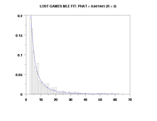
LOST GAMES MAXIMUM LIKELIHOOD Y2 X2


The maximum likelihood estimate of p is

with denoting the sample mean.

For a given value of r, generate an estimate of p based on the maximum ppcc value or the minimum chi-square goodness of fit with the commands

LET R = <value>
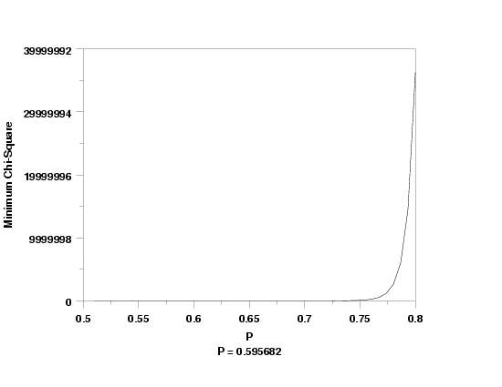
LET P1 = <value>
LET P2 = <value>
LOST GAMES KS PLOT Y
LOST GAMES KS PLOT Y2 X2
LOST GAMES KS PLOT Y3 XLOW XHIGH
LOST GAMES PPCC PLOT Y
LOST GAMES PPCC PLOT Y2 X2
LOST GAMES PPCC PLOT Y3 XLOW XHIGH


The default values of P1 and P2 are 0.51 and 0.95, respectively. The value of R should typically be set to the minimum value of the data. Due to the discrete nature of the percent point function for discrete distributions, the ppcc plot will not be smooth. For that reason, if there is sufficient sample size the KS PLOT (i.e., the minimum chi-square value) is typically preferred. Also, since the data is integer values, one of the binned forms is preferred for these commands.

None

None

LOSCDF	= Compute the lost games cumulative distribution function.
LOSPPF	= Compute the lost games percent point function.
BTAPDF	= Compute the Borel-Tanner probability mass function.
POIPDF	= Compute the Poisson probability mass function.
HERPDF	= Compute the Hermite probability mass function.
BINPDF	= Compute the binomial probability mass function.
NBPDF	= Compute the negative binomial probability mass function.
GEOPDF	= Compute the geometric probability mass function.
INTEGER FREQUENCY TABLE	= Generate a frequency table at integer values with unequal bins.
COMBINE FREQUENCY TABLE	= Convert an equal width frequency table to an unequal width frequency table.
KS PLOT	= Generate a minimum chi-square plot.
MAXIMUM LIKELIHOOD	= Perform maximum likelihood estimation for a distribution.

Luc Devroye (1986), "Non-Uniform Random Variate Generation", Springer-Verlang, pp. 758-759.

Kemp and Kemp (1968), "On a Distribution Associated with Certain Stochastic Processes", Journal of the Royal Statistical Society, Series B, 30, pp. 401-410.

Haight (1961), "A Distribution Analogous to the Borel-Tanner Distribution", Biometrika, 48, pp. 167-173.

Johnson, Kotz, and Kemp (1992), "Univariate Discrete Distributions", Second Edition, Wiley, pp. 445-447.

Distributional Modeling

2006/6

 
let r = 3
let p = 0.6
let y = lost games random numbers for i = 1 1 500
.
let y3 xlow xhigh = integer frequency table y
class lower 1.5
class width 1
let amax = maximum y
let amax2 = amax + 0.5
class upper amax2
let y2 x2 = binned y
.
let k = minimum y
lost games mle y
let p = pml
lost games chi-square goodness of fit y3 xlow xhigh
relative histogram y2 x2
limits freeze
pre-erase off
line color blue
title Lost Games MLE FIt: Phat = ^pml (r = ^r)
plot lospdf(x,pml,r) for x = r  1  amax
title
limits
pre-erase on
line color black
.
label case asis
x1label P
y1label Minimum Chi-Square
let p1 = 0.5
let p2 = 0.9
lost games ks plot y3 xlow xhigh
let p = shape
case asis
justification center
move 50 5
text P = ^p
lost games chi-square goodness of fit y3 xlow xhigh
    



           LOST GAMES MAXIMUM LIKELIHOOD ESTIMATION:
  
 NUMBER OF OBSERVATIONS                   =      500
 SAMPLE MEAN                              =    8.892000
 SAMPLE STANDARD DEVIATION                =    8.214822
 SAMPLE MINIMUM                           =    3.000000
 SAMPLE MAXIMUM                           =    62.00000
  
 ESTIMATE OF R                            =    3.000000
 MAXIMUM LIKELIHOOD ESTIMATE OF P         =   0.6014611
  
 THE MAXIMUM LIKELIHOOD ESTIMATES FOR R AND P
 ARE SAVED IN THE INTERNAL PARAMETERS RML AND PML
  
  
 THE COMPUTED VALUE OF THE CONSTANT P        =   0.6014611E+00
  
  
                   CHI-SQUARED GOODNESS-OF-FIT TEST
  
 NULL HYPOTHESIS H0:      DISTRIBUTION FITS THE DATA
 ALTERNATE HYPOTHESIS HA: DISTRIBUTION DOES NOT FIT THE DATA
 DISTRIBUTION:            LOST GAMES
  
 SAMPLE:
    NUMBER OF OBSERVATIONS      =      500
    NUMBER OF NON-EMPTY CELLS   =       24
    NUMBER OF PARAMETERS USED   =        2
  
 TEST:
 CHI-SQUARED TEST STATISTIC     =    22.46355
    DEGREES OF FREEDOM          =       21
    CHI-SQUARED CDF VALUE       =    0.626767
  
    ALPHA LEVEL         CUTOFF              CONCLUSION
            10%       29.61509               ACCEPT H0
             5%       32.67057               ACCEPT H0
             1%       38.93217               ACCEPT H0
  
       CELL NUMBER, LOWER BIN POINT, UPPER BIN POINT, OBSERVED FREQUENCY, AND EXPECTED FREQUENCY
       WRITTEN TO FILE DPST1F.DAT
    



                   CHI-SQUARED GOODNESS-OF-FIT TEST
  
 NULL HYPOTHESIS H0:      DISTRIBUTION FITS THE DATA
 ALTERNATE HYPOTHESIS HA: DISTRIBUTION DOES NOT FIT THE DATA
 DISTRIBUTION:            LOST GAMES
  
 SAMPLE:
    NUMBER OF OBSERVATIONS      =      500
    NUMBER OF NON-EMPTY CELLS   =       24
    NUMBER OF PARAMETERS USED   =        2
  
 TEST:
 CHI-SQUARED TEST STATISTIC     =    21.82713
    DEGREES OF FREEDOM          =       21
    CHI-SQUARED CDF VALUE       =    0.590470
  
    ALPHA LEVEL         CUTOFF              CONCLUSION
            10%       29.61509               ACCEPT H0
             5%       32.67057               ACCEPT H0
             1%       38.93217               ACCEPT H0
  
       CELL NUMBER, LOWER BIN POINT, UPPER BIN POINT, OBSERVED FREQUENCY, AND EXPECTED FREQUENCY
       WRITTEN TO FILE DPST1F.DAT