SED navigation bar go to SED home page go to Dataplot home page go to NIST home page SED Home Page SED Staff SED Projects SED Products and Publications Search SED Pages
Dataplot Vol 2 Vol 1

PERCENTAGE BEND MIDVARIANCE

Name:
    PERCENTAGE BEND MIDVARIANCE (LET)
Type:
    Let Subcommand
Purpose:
    Compute the percentage bend midvariance for a variable.
Description:
    Mosteller and Tukey (see Reference section below) define two types of robustness:

    1. resistance means that changing a small part, even by a large amount, of the data does not cause a large change in the estimate

    2. robustness of efficiency means that the statistic has high efficiency in a variety of situations rather than in any one situation. Efficiency means that the estimate is close to optimal estimate given that we know what distribution that the data comes from. A useful measure of efficiency is:

        Efficiency = (lowest variance feasible)/ (actual variance)

    Many statistics have one of these properties. However, it can be difficult to find statistics that are both resistant and have robustness of efficiency.

    For scale estimaors, the variance is an optimal estimator for Gaussian data. However, it is not resistant and it does not have robustness of efficiency. The rationale for this estimate is given in these references.

    The percentage bend midvariance estimator, discussed in Shoemaker and Hettmansperger and also by Wilcox, is both resistant and robust of efficiency.

    The percentage bend midvariance of a a variable X is computed as follows:

    1. Set m = [(1 - \( \beta \) )*n + 0.5]. This is the value of (1 - \( \beta \) )*n + 0.5 rounded down to the nearest integer.

    2. Let Wi = |Xi - M| for i = 1, ..., n where M is the median of X.

    3. Sort the Wi in ascending order.

    4. \( \hat{W}_{x} \) = W(m) (i. e., the m-th order statistic). W(m) is the estimate of the (1-\( \beta \)) quantile of W.

    5. \( Y_i = \frac{X_i - M}{\hat{\omega}_{\beta}} \)

    6. \( A(i) = \log(x_{i}) \)

    7. \( \Psi(x) = \max[-1, \min(1,x)] \)

    8. \( s_{pb} = \frac {n \hat{\omega}_{\beta} \sum_{i=1}^{n}{ \left( \Psi(Y_{i}) \right) ^2} } {(\sum_{i=1}^{n}{a_{i}})^{2} } \)

    The value of \( \beta \) is selected between 0 and 0.5. Higher values of \( \beta \) is selected result in a higher breakdown point at the expense of lower efficiency.

Syntax:
    LET <par> = PERCENTAGE BEND MIDVARIANCE <y>        <SUBSET/EXCEPT/FOR qualification>
    where <y> is the response variable;
                  <par> is a parameter where the computed percentage bend midvariance is stored;
    and where the <SUBSET/EXCEPT/FOR qualification> is optional.
Examples:
    LET A = PERCENTAGE BEND MIDVARIANCE Y1
    LET A = PERCENTAGE BEND MIDVARIANCE Y1 SUBSET TAG > 2
Note:
    To set the value of \( \beta \), enter the command

      LET BETA = <value>

    where <value> is greater than 0 and less than or equal to 0.5. The default value for \( \beta \) is 0.1.

Note:
    Dataplot statistics can be used in a number of commands. For details, enter

Default:
    None
Synonyms:
    None
Related Commands: References:
    Shoemaker and Hettmansperger (1982), "Robust Estimates of and Tests for the One- and Two-Sample Scale Models", Biometrika 69, pp. 47-54.

    Rand Wilcox (1997), "Introduction to Robust Estimation and Hypothesis Testing", Academic Press.

    Mosteller and Tukey (1977), "Data Analysis and Regression: A Second Course in Statistics", Addison-Wesley, pp. 203-209.

Applications:
    Robust Data Analysis
Implementation Date:
    2002/07
Program 1:
     
    LET Y1 = NORMAL RANDOM NUMBERS FOR I = 1 1 100
    LET Y2 = LOGISTIC RANDOM NUMBERS FOR I = 1 1 100
    LET Y3 = CAUCHY RANDOM NUMBERS FOR I = 1 1 100
    LET Y4 = DOUBLE EXPONENTIAL RANDOM NUMBERS FOR I = 1 1 100
    LET A1 = PERCENTAGE BEND MIDVARIANCE Y1
    LET A2 = PERCENTAGE BEND MIDVARIANCE Y2
    LET A3 = PERCENTAGE BEND MIDVARIANCE Y3
    LET A4 = PERCENTAGE BEND MIDVARIANCE Y4
        
Program 2:
     
    MULTIPLOT 2 2
    MULTIPLOT CORNER COORDINATES 0 0 100 100
    MULTIPLOT SCALE FACTOR 2
    X1LABEL DISPLACEMENT 12
    .
    LET Y1 = NORMAL RANDOM NUMBERS FOR I = 1 1 200
    LET Y2 = CAUCHY RANDOM NUMBERS FOR I = 1 1 200
    .
    BOOTSTRAP SAMPLES 500
    BOOTSTRAP PERCENTAGE BEND MIDVARIANCE PLOT Y1
    X1LABEL B025 = ^B025, B975=^B975
    HISTOGRAM YPLOT
    X1LABEL
    .
    BOOTSTRAP PERCENTAGE BEND MIDVARIANCE PLOT Y1
    X1LABEL B025 = ^B025, B975=^B975
    HISTOGRAM YPLOT
    .
    END OF MULTIPLOT
    JUSTIFICATION CENTER
    MOVE 50 96
    TEXT PERCENTAGE BEND MIDVARIANCE BOOTSTRAP: NORMAL
    MOVE 50 46
    TEXT PERCENTAGE BEND MIDVARIANCE BOOTSTRAP: CAUCHY
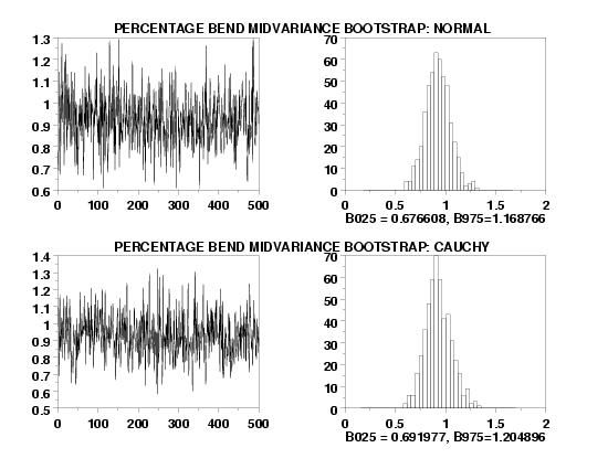
        
    plot generated by sample program

Privacy Policy/Security Notice
Disclaimer | FOIA

NIST is an agency of the U.S. Commerce Department.

Date created: 07/22/2002
Last updated: 10/07/2016

Please email comments on this WWW page to alan.heckert@nist.gov.