SED navigation bar go to SED home page go to Dataplot home page go to NIST home page SED Home Page SED Staff SED Projects SED Products and Publications Search SED Pages
Dataplot Vol 2 Vol 1

PEXPDF

Name:
    PEXPDF (LET)
Type:
    Library Function
Purpose:
    Compute the exponential power probability density function with shape parameter beta.
Description:
    The exponential power distribution has the following probability density function:

      f(x;beta) = beta*x^(beta-1)*EXP(x^beta)*EXP(1 - EXP(x^beta))    
x > 0; beta > 0

    with beta denoting the shape parameter.

    This distribution can be generalized with location and scale parameters using the relation

      f(x;beta,loc,scale) = (1/scale)*f((x-loc)/scale;beta,0,1)

    This distribution was proposed by Dhillon as useful distribution for reliability applications since it can have increasing, decreasing, or bathtub shaped hazard functions.

Syntax:
    LET <y> = PEXPDF(<x>,<beta>,<loc>,<scale>)
                            <SUBSET/EXCEPT/FOR qualification>
    where <x> is a number, parameter, or variable containing positive values;
                <y> is a variable or a parameter (depending on what <x> is) where the computed exponential power pdf value is stored;
                <beta> is a positive number, parameter, or variable that specifies the shape parameter;
                <loc> is a number, parameter, or variable that specifies the location parameter;
                <scale> is a positive number, parameter, or variable that specifies the scale parameter;
    and where the <SUBSET/EXCEPT/FOR qualification> is optional.

    If <loc> and <scale> are omitted, they default to 0 and 1, respectively.

Examples:
    LET A = PEXPDF(0.3,2.5)
    LET A = PEXPDF(X1,2.5,0,10)
    PLOT PEXPDF(X,2.5,0,3) FOR X = 0.1 0.1 10
Note:
    The 11/2007 version changed the syntax for this function from

      LET A = PEXPDF(X,ALPHA,BETA,LOC,SCALE)

    to

      LET A = PEXPDF(X,BETA,LOC,SCALE)

    This was done since ALPHA is in fact a scale parameter (in the articles listed in the References section, ALPHA is actually the reciprocal of the scale parameter).

Note:
    Exponential power random numbers, probability plots, and goodness of fit tests can be generated with the commands:

      LET BETA = <value>
      LET Y = EXPONENTIAL POWER RANDOM NUMBERS FOR I = 1 1 N
      EXPONENTIAL POWER PROBABILITY PLOT Y
      EXPONENTIAL POWER PROBABILITY PLOT Y2 X2
      EXPONENTIAL POWER PROBABILITY PLOT Y3 XLOW XHIGH
      EXPONENTIAL POWER KOLMOGOROV SMIRNOV ...
                  GOODNESS OF FIT Y
      EXPONENTIAL POWER CHI-SQUARE GOODNESS OF FIT ...
                  Y2 X2
      EXPONENTIAL POWER CHI-SQUARE GOODNESS OF FIT ...
                  Y3 XLOW XHIGH

    The following commands can be used to estimate the beta shape parameter for the exponential power distribution:

      LET BETA1 = <value>
      LET BETA2 = <value>
      EXPONENTIAL POWER PPCC PLOT Y
      EXPONENTIAL POWER PPCC PLOT Y2 X2
      EXPONENTIAL POWER PPCC PLOT Y3 XLOW XHIGH
      EXPONENTIAL POWER KS PLOT Y
      EXPONENTIAL POWER KS PLOT Y2 X2
      EXPONENTIAL POWER KS PLOT Y3 XLOW XHIGH

    The default values for BETA1 and BETA2 are 0.5 and 10.

    The probability plot can then be used to estimate the location and scale (location = PPA0, scale = PPA1).

    The 2-parameter exponential power maximum likelihood estimates can be obtained using the command

      EXPONENTIAL POWER MAXIMUM LIKELIHOOD Y

    The maximum likelihood estimates are the solution of the following simultaneous equations:

      (n/beta) + n*LOG(alpha) + SUM[i=1 to n][A(i)] - 
SUM[i=1 to n][B(i)*C(i)*EXP(B(i))] + SUM[i=1 to n][B(i)*C(i)] = 0

      (beta*n/alpha) - (beta/alpha)*SUM[i=1 to n][B(i)*EXP(B(i))] + 
SUM[i=1 to n][B(i)] = 0

    where

      alpha = 1/scale

      A(i) = LOG(X(i))

      B(i) = (alpha*X(i))^beta

      C(i) = LOG(alpha*X(i))

    The standard error of beta is

      -(n/beta^2) - SUM[i=1 to n][C(i)^2*B(i)*(B(i)+1)*EXP(B(i))] + 
SUM[i=1 to n][C(i)^2*B(i)]

    The standard error of alpha (= 1/scale) is

      -(beta*n/alpha^2) - 
(beta/alpha^2)*SUM[i=1 to n][EXP(B(i))*((beta-1)*B(i) + B(i)^2*beta)] + 
(beta*(beta-1)/alpha^2)*SUM[i=1 to n][B(i)]

    The covariance of beta and alpha is

      (n/alpha) - 
(1/alpha)*SUM[i=1 to n][B(i)*EXP(B(i))*(1+beta*LOG(alpha)+beta*A(i)+
beta*B(i)*C(i)} + 
(1/alpha)*SUM[i=1 to n][B(i)*(1+beta*LOG(alpha)+beta*A(i))}

    The above equations are from the Dhillon paper.

    Our experience indicates that the maximum likelihood can fail, particularly when the scale parameter is > 1. Specifying improved starting values can sometimes help (for example, use the estimates obtained from the ppcc/ probability plot method as starting values). These can be specified with the commands

      LET ALPHASV = <value>
      LET BETASV = <value>

    In this context, ALPHASV is the starting value for the scale parameter, not the reciprocal of the scale parameter.

    The BOOTSTRAP DISTRIBUTION command can be used to find uncertainty intervals for the ppcc plot and the ks plot methods. Bootstrap confidence intervals are currently not supported for the maximum likelihood method.

Default:
    None
Synonyms:
    None
Related Commands:
    PEXCDF = Compute the exponential power cumulative distribution function.
    PEXPPF = Compute the exponential power percent point function.
    PEXHAZ = Compute the exponential power hazard function.
    PEXCHAZ = Compute the exponential power cumulative hazard function.
    ALPPDF = Compute the alpha probability density function.
    WEIPDF = Compute the Weibull probability density function.
    LGNPDF = Compute the log-normal probability density function.
    NORPDF = Compute the normal probability density function.
References:
    Johnson, Kotz, and Balakrishnan (1994), "Continuous Univariate Distributions--Volume 2", Second Edition, John Wiley and Sons, pp. 643-644.

    Dhillon (1981), "Life Distributions", IEEE Transactions on Reliability, Vol. R-30, No. 5, pp. 457-459.

Applications:
    Reliability, accelerated life testing
Implementation Date:
    1998/4
    2007/11: Corrected the second shape parameter to be the scale parameter
Program 1:
     
    LABEL CASE ASIS
    TITLE CASE ASIS
    TITLE OFFSET 2
    .
    MULTIPLOT 2 2
    MULTIPLOT CORNER COORDINATES 0 0 100 95
    MULTIPLOT SCALE FACTOR 2
    .
    LET BETA  = 0.5
    TITLE BETA = ^beta
    PLOT PEXPDF(X,BETA) FOR X = 0.01  0.01  2
    .
    LET BETA  = 1
    TITLE BETA = ^beta
    PLOT PEXPDF(X,BETA) FOR X = 0.01  0.01  2
    .
    LET BETA  = 2
    TITLE BETA = ^beta
    PLOT PEXPDF(X,BETA) FOR X = 0.01  0.01  2
    .
    LET BETA  = 5
    TITLE BETA = ^beta
    PLOT PEXPDF(X,BETA) FOR X = 0.01  0.01  2
    .
    END OF MULTIPLOT
    .
    JUSTIFICATION CENTER
    MOVE 50 97
    TEXT Exponential Power Probability Density Functions
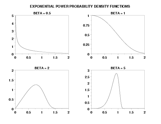
        
    plot generated by sample program
Program 2:
     
    let beta = 2.4
    let y = exponential power random numbers for i = 1 1 200
    let y = 0.6*y
    let betasav = beta
    let amax = maximum y
    .
    exponential power ppcc plot y
    let beta1 = beta - 1
    let beta1 = max(beta1,0.1)
    let beta2 = beta + 1
    y1label Correlation Coefficient
    x1label Beta
    exponential power ppcc plot y
    justification center
    move 50 6
    let beta = shape
    text Betahat = ^beta (True Value: ^betasav)
    .
    char x
    line bl
    y1label Data
    x1label Theoretical
    exponential power prob plot y
    move 50 6
    text Location = ^ppa0, Scale = ^ppa1
    move 50 2
    text PPCC = ^ppcc
    char bl
    line so
    label
    .
    relative histogram y
    limits freeze
    pre-erase off
    plot pexpdf(x,beta,ppa0,ppa1) for x = 0.01 .01 amax
    limits 
    pre-erase on
    .
    let ksloc = ppa0
    let ksscale = ppa1
    exponential power kolm smir goodness of fit y
    .
    exponential power mle y
    .
    let beta = betaml
    let ksloc = ppa0
    let ksscale = alphaml
    exponential power kolm smir goodness of fit y
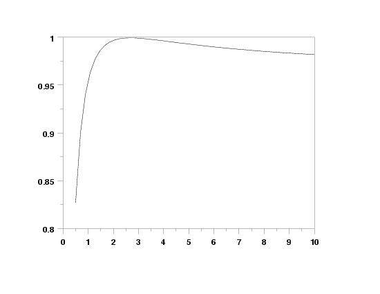
        
    plot generated by sample program

    plot generated by sample program

    plot generated by sample program

    plot generated by sample program

                       KOLMOGOROV-SMIRNOV GOODNESS-OF-FIT TEST
      
     NULL HYPOTHESIS H0:      DISTRIBUTION FITS THE DATA
     ALTERNATE HYPOTHESIS HA: DISTRIBUTION DOES NOT FIT THE DATA
     DISTRIBUTION:            EXPONENTIAL POWER
        NUMBER OF OBSERVATIONS              =      200
      
     TEST:
     KOLMOGOROV-SMIRNOV TEST STATISTIC      =   0.3395832E-01
      
        ALPHA LEVEL         CUTOFF              CONCLUSION
                10%       0.086*              ACCEPT H0
                          0.085**
                 5%       0.096*              ACCEPT H0
                          0.095**
                 1%       0.115*              ACCEPT H0
                          0.114**
      
         *  - STANDARD LARGE SAMPLE APPROXIMATION  ( C/SQRT(N) )
        ** - MORE ACCURATE LARGE SAMPLE APPROXIMATION  ( C/SQRT(N + SQRT(N/10)) )
     
    
           EXPONENTIAL POWER PARAMETER ESTIMATION: FULL SAMPLE CASE
                 TWO-PARAMETER MODEL (LOCATION = 0)
      
     SUMMARY STATISTICS:
     NUMBER OF OBSERVATIONS                            =      200
     SAMPLE MEAN                                       =   0.4626617
     SAMPLE STANDARD DEVIATION                         =   0.1564132
     SAMPLE MINIMUM                                    =   0.3986295E-01
     SAMPLE MAXIMUM                                    =   0.7760341
      
     MAXIMUM LIKELIHOOD ESTIMATES:
     ESTIMATE OF SHAPE PARAMETER                       =    2.529571
     STANDARD ERROR OF SHAPE PARAMETER                 =   0.1515455
     ESTIMATE OF SCALE PARAMETER                       =   0.6117715
     STANDARD ERROR OF SCALE PARAMETER                 =   0.2820683E-01
     COVARIANCE OF SHAPE/SCALE PARAMETERS              =  -0.7626695E-03
      
     CONFIDENCE INTERVAL FOR SCALE PARAMETER
      
                            NORMAL APPROXIMATION
        CONFIDENCE           LOWER         UPPER
        VALUE (%)            LIMIT         LIMIT
     -------------------------------------------
          50.000          0.592746      0.630797
          75.000          0.579324      0.644219
          90.000          0.565375      0.658168
          95.000          0.556487      0.667056
          99.000          0.539115      0.684427
          99.900          0.518957      0.704586
      
     CONFIDENCE INTERVAL FOR SHAPE PARAMETER
                            NORMAL APPROXIMATION
        CONFIDENCE           LOWER         UPPER
        VALUE (%)            LIMIT         LIMIT
     -------------------------------------------
          50.000           2.42736       2.63179
          75.000           2.35524       2.70390
          90.000           2.28030       2.77884
          95.000           2.23255       2.82659
          99.000           2.13922       2.91993
          99.900           2.03091       3.02823
      
      
                       KOLMOGOROV-SMIRNOV GOODNESS-OF-FIT TEST
      
     NULL HYPOTHESIS H0:      DISTRIBUTION FITS THE DATA
     ALTERNATE HYPOTHESIS HA: DISTRIBUTION DOES NOT FIT THE DATA
     DISTRIBUTION:            EXPONENTIAL POWER
        NUMBER OF OBSERVATIONS              =      200
      
     TEST:
     KOLMOGOROV-SMIRNOV TEST STATISTIC      =   0.2892238E-01
      
        ALPHA LEVEL         CUTOFF              CONCLUSION
                10%       0.086*              ACCEPT H0
                          0.085**
                 5%       0.096*              ACCEPT H0
                          0.095**
                 1%       0.115*              ACCEPT H0
                          0.114**
      
         *  - STANDARD LARGE SAMPLE APPROXIMATION  ( C/SQRT(N) )
        ** - MORE ACCURATE LARGE SAMPLE APPROXIMATION  ( C/SQRT(N + SQRT(N/10)) )


Date created: 11/27/2007
Last updated: 11/27/2007
Please email comments on this WWW page to alan.heckert@nist.gov.