
|
|
STPPFName:

with
For The skew-t percent point function is computed numerically (by inverting the skew-t cdf function with the bisection method). The standard skew-t distribution can be generalized with location and scale parameters.
<SUBSET/EXCEPT/FOR qualification> where <p> is a variable or a parameter in the range [0,1]; <nu> is a number of parameter that specifies the value of the degrees of freedom shape parameter; <lambda> is a number of parameter that specifies the value of the skewness shape parameter; <y> is a variable or a parameter (depending on what <p> is) where the computed skew-t ppf value is stored; and where the <SUBSET/EXCEPT/FOR qualification> is optional.
LET A = STPPF(A1,DF,LAMBDA) LET X2 = STPPF(P1,NU,0.5)
"Log-Skew-Normal and Log-Skew-t Distributions as Models for Familiy Income Data", Azzalini and Dal Cappello, unpublished paper downloaded from Azzallini web site.
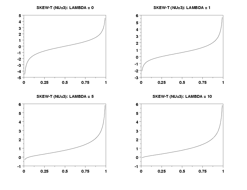
MULTIPLOT 2 2
MULTIPLOT CORNER COORDINATES 0 0 100 100
TITLE SKEW-T (NU=3): LAMBDA = 0
PLOT STPPF(P,3,0) FOR P = 0.01  0.01  0.99
TITLE SKEW-T (NU=3): LAMBDA = 1
PLOT STPPF(P,3,1) FOR P = 0.01  0.01  0.99
TITLE SKEW-T (NU=3): LAMBDA = 5
PLOT STPPF(P,3,5) FOR P = 0.01  0.01  0.99
TITLE SKEW-T (NU=3): LAMBDA = 10
PLOT STPPF(P,3,10) FOR P = 0.01  0.01  0.99
END OF MULTIPLOT
Date created: 2/3/2004 |
 ,
,
 ,
TCDF, and TPDF denoting the degrees of freedom parameter,
the skewness parameter, the cumulative distribution function
of the t distribution, and the probability density
function of the t distribution, respectively.
,
TCDF, and TPDF denoting the degrees of freedom parameter,
the skewness parameter, the cumulative distribution function
of the t distribution, and the probability density
function of the t distribution, respectively.