TSOPDF

TSOPDF (LET)

Library Function

Compute the two-sided ogive probability density function with shape parameters n and .

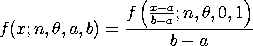
The standard two-sided ogive distribution has the following probability density function:

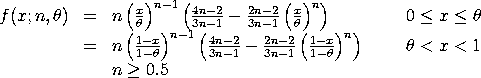
with n denoting the shape parameter and denoting the reflection parameter.

This distribution can be extended with lower and upper bound parameters. If a and b denote the lower and upper bounds, respectively, then the location and scale parameters are:

location = a
scale = b - a


The general form of the distribution can then be found by using the relation

Kotz and Van Dorp note that the two-sided ogive distribution is smooth at the reflection point (x = ). This is in contrast to the two-sided slope and two-sided power distributions, which are not smooth at the relection point.

LET <y> = TSOPDF(<x>,<n>,<theta>,<a>,<b>)
                        <SUBSET/EXCEPT/FOR qualification>
where <x> is a number, parameter, or variable containing values in the interval (a,b);
            <y> is a variable or a parameter (depending on what <x> is) where the computed two-sided ogive pdf value is stored;
            <n> is a number, parameter, or variable in the interval (≥ 0.5) that specifies the first shape parameter;
            <theta> is a number, parameter, or variable in the interval (a,b) that specifies the second shape parameter;
            <a> is a number, parameter, or variable that specifies the lower bound;
            <b> is a number, parameter, or variable that specifies the upper bound;
and where the <SUBSET/EXCEPT/FOR qualification> is optional.

If <a> and <b> are omitted, they default to 0 and 1, respectively.

LET A = TSOPDF(0.3,1.2,0.3)
LET Y = TSOPDF(X,1.5,2.2,0,5)
PLOT TSOPDF(X,1.5,2.2,0,5) FOR X = 0 0.01 5

Two-sided slope random numbers, probability plots, and goodness of fit tests can be generated with the commands:
LET THETA = <value>
LET N = <value>
LET A = <value>
LET B = <value>
LET Y = TWO-SIDED SLOPE RANDOM NUMBERS FOR I = 1 1 N
TWO-SIDED SLOPE PROBABILITY PLOT Y
TWO-SIDED SLOPE PROBABILITY PLOT Y2 X2
TWO-SIDED SLOPE PROBABILITY PLOT Y3 XLOW XHIGH
TWO-SIDED SLOPE KOLMOGOROV SMIRNOV GOODNESS OF FIT Y
TWO-SIDED SLOPE CHI-SQUARE GOODNESS OF FIT Y2 X2
TWO-SIDED SLOPE CHI-SQUARE GOODNESS OF FIT Y3 XLOW XHIGH


Note that

A ≤ data minimum < THETA < data maximum ≤ B

The following commands can be used to estimate the n and shape parameters for the two-sided ogive distribution:

LET A = <value>
LET B = <value>
LET THETA1 = <value>
LET THETA2 = <value>
LET N1 = <value>
LET N2 = <value>
TWO-SIDED SLOPE PPCC PLOT Y
TWO-SIDED SLOPE PPCC PLOT Y2 X2
TWO-SIDED SLOPE PPCC PLOT Y3 XLOW XHIGH
TWO-SIDED SLOPE KS PLOT Y
TWO-SIDED SLOPE KS PLOT Y2 X2
TWO-SIDED SLOPE KS PLOT Y3 XLOW XHIGH


Note that for the two-sided ogive distribution, the shape parameter is bounded by the minimum and maximum of the data. In the above commands, there are two approaches to dealing with this.

1. Specify the values for A and B (i.e., the LET A = and LET B = commands).

   The advantage of this approach is that is estimated in units of the data. The disadvantage is that we lose the invariance of location and scale for the PPCC plot (i.e., we cannot obtain estimates of A and B).

2. Use A = 0 and B = 1 (i.e., the standard form of the distribution). This restricts the value of to the (0,1) interval.

   The advantage of this approach is that we maintain the invariance of location and scale for the PPCC plot and can obtain indpendent estimates for A and B.

   The disadvantage of this approach is that we have to scale the estimate of if the data are outside of the (0,1) interval.

   To scale the estimate of in this method, do something like the following:

   DELETE A B
   LET YMIN = MINIMUM Y
   LET YMAX = MAXIMUM Y
   TWO-SIDED OGIVE PPCC PLOT Y
   LET N = SHAPE1
   LET THETA = SHAPE2
   TWO SIDED OGIVE PROBABILITY PLOT Y
   LET A = PPA0
   LET B = A + PPA1
   LET A = MIN(A,YMIM)
   LET B = MAX(B,YMAX)
   LET THETA = A + (B-A)*THETA
   

   We include a check to make sure that the estimated values for A and B are permissable (i.e., A ≤ YMIN and B ≥ YMAX).

The default values for N1 and N2 are 0.05 and 10.

None

None

TSOCDF	= Compute the two-sided ogive cumulative distribution function.
TSOPPF	= Compute the two-sided ogive percent point function.
OGIPDF	= Compute the ogive probability density function.
TSSPDF	= Compute the two-sided slope probability density function.
TSPPDF	= Compute the two-sided power probability density function.
POWPDF	= Compute the power probability density function.
SLOPDF	= Compute the slope probability density function.
BETPDF	= Compute the Beta probability density function.
JSBPDF	= Compute the Johnson SB probability density function.

Samuel Kotz and J. Rene Van Dorp 2004, "Beyond N: Other Continuous Families of Distributions with Bounded Support and Applications", World Scientific, chapter 8.

Distributional modeling

2007/10

 
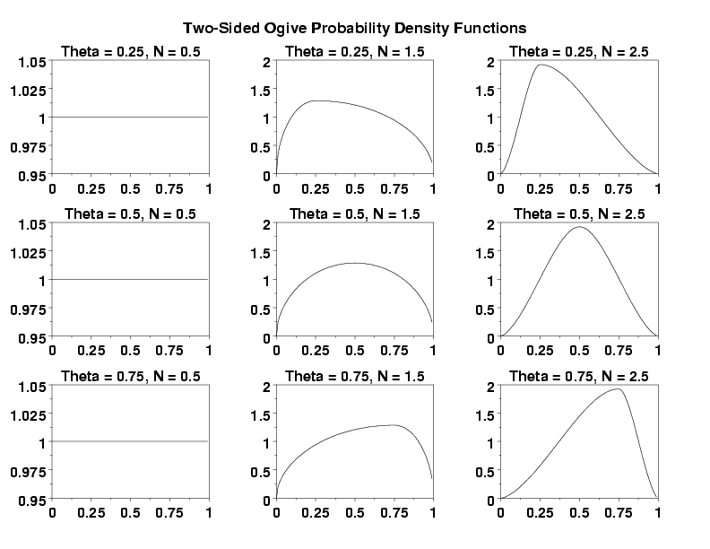
MULTIPLOT 3 3
MULTIPLOT CORNER COORDINATES 0 0 100 95
MULTIPLOT SCALE FACTOR 3
TITLE OFFSET 2
TITLE CASE ASIS
LABEL CASE ASIS
CASE ASIS
.
LET THETAV = DATA 0.25  0.50 0.75
LET NV = DATA 0.5  1.0  1.5
.
LOOP FOR K = 1 1 3
   LET THETA = THETAV(K)
   LOOP FOR L = 1 1 3
      LET N = NV(L)
      TITLE Theta = ^THETA, Alpha = ^N
      PLOT TSOPDF(X,N,THETA) FOR X = 0  0.01  1
   END OF LOOP
END OF LOOP
.
END OF MULTIPLOT
MOVE 50 97
JUSTIFICATION CENTER
TEXT Two-Sided Ogive Probability Density Functions
    

    
       
    
    

    

 
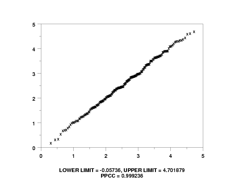
let n = 2.3
let theta = 2.5
let a = 0
let b = 5
let nsv = n
let thetasv = theta
.
let y = two-sided ogive rand numb for i = 1 1 200
let ymin = minimum y
let ymax = maximum y
.
let theta1 = 1.5
let theta2 = 4
let n1 = 1.1
let n2 = 5
two-sided ogive ppcc plot y
let n = shape1
let theta = shape2
justification center
move 50 6
text Thetahat = ^theta, ^Nhat = ^n
move 50 3
text Theta = ^thetasv, N = ^Nsv
.
character x
line bl
two-sided ogive probability plot y
let a = ppa0
let b = ppa0 + ppa1
let a = min(a,ymin)
let b = max(b,ymax)
move 50 6
text Lower Limit = ^a, Upper Limit = ^b
move 50 3
text PPCC = ^ppcc
char bl
line so
.
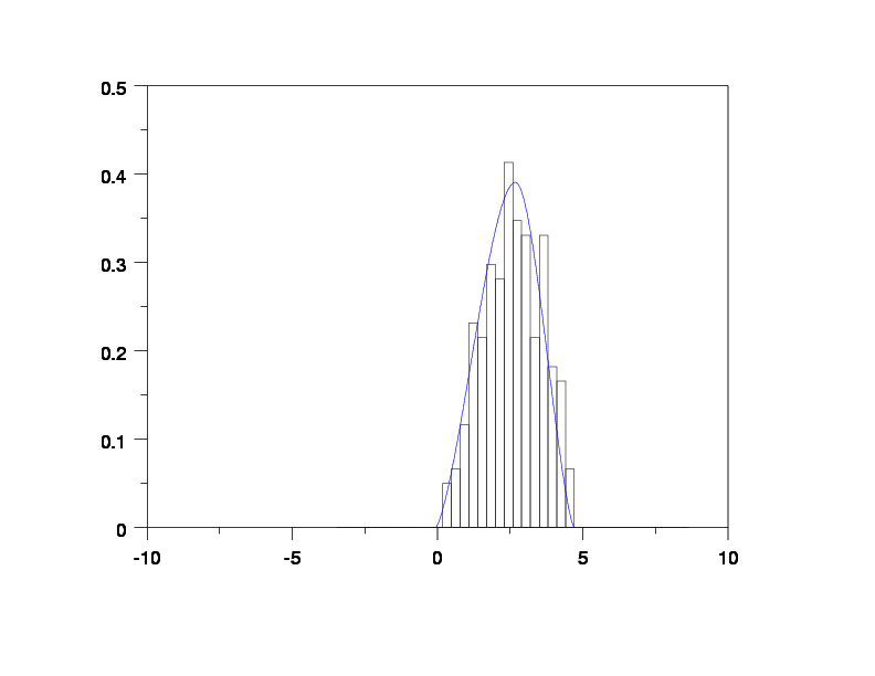
let ksloc = ppa0
let ksscale = (b-a)
two-sided ogive kolm smir goodness of fit y
.
relative hist y
line color blue
limits freeze
pre-erase off
plot tsopdf(x,n,theta,a,b) for x = a 0.01 b
limits
pre-erase on
line color black all
    







                   KOLMOGOROV-SMIRNOV GOODNESS-OF-FIT TEST
  
 NULL HYPOTHESIS H0:      DISTRIBUTION FITS THE DATA
 ALTERNATE HYPOTHESIS HA: DISTRIBUTION DOES NOT FIT THE DATA
 DISTRIBUTION:            TWO-SIDED OGIVE
    NUMBER OF OBSERVATIONS              =      200
  
 TEST:
 KOLMOGOROV-SMIRNOV TEST STATISTIC      =   0.8571517E-01
  
    ALPHA LEVEL         CUTOFF              CONCLUSION
            10%       0.086*              REJECT H0
                      0.085**
             5%       0.096*              ACCEPT H0
                      0.095**
             1%       0.115*              ACCEPT H0
                      0.114**
  
     *  - STANDARD LARGE SAMPLE APPROXIMATION  ( C/SQRT(N) )
    ** - MORE ACCURATE LARGE SAMPLE APPROXIMATION  ( C/SQRT(N + SQRT(N/10)) )