8. Assessing Product Reliability
8.4. Reliability Data Analysis
8.4.2. How do you fit an acceleration model?

8.4.2.3.

Fitting models using degradation data instead of failures

If you can fit models using degradation data, you don't need actual test failures

When failure can be related directly to a change over time in a measurable product parameter, it opens up the possibility of measuring degradation over time and using that data to extrapolate when failure will occur. That allows us to fit acceleration models and life distribution models without actually waiting for failures to occur.

This overview of degradation modeling assumes you have chosen a life distribution model and an acceleration model and offers an alternative to the accelerated testing methodology based on failure data, previously described. The following topics are covered.

• Common assumptions
• Advantages
• Drawbacks
• A simple method
• A more accurate approach for a special case
• Example

More details can be found in Nelson (1990, pages 521-544) or Tobias and Trindade (1995, pages 197-203).

Common Assumptions When Modeling Degradation Data

You need a measurable parameter that drifts (degrades) linearly to a critical failure value

Two common assumptions typically made when degradation data are modeled are the following:

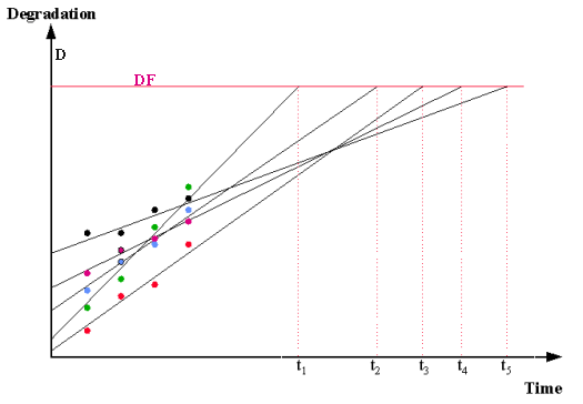
1. A parameter \(D\), that can be measured over time, drifts monotonically (upwards, or downwards) towards a specified critical value \(DF\). When it reaches \(DF\), failure occurs.
2. The drift, measured in terms of \(D\), is linear over time with a slope (or rate of degradation) \(R\), that depends on the relevant stress the unit is operating under and also the (random) characteristics of the unit being measured. Note: It may be necessary to define \(D\) as a transformation of some standard parameter in order to obtain linearity - logarithms or powers are sometimes needed.

The figure below illustrates these assumptions by showing degradation plots of five units on test. Degradation readings for each unit are taken at the same four time points and straight lines fit through these readings on a unit-by-unit basis. These lines are then extended up to a critical (failure) degradation value. The projected times of failure for these units are then read off the plot. The are: \(t_1, \, t_2, \, \ldots, \, t_5\).

Plot of linear degradation trends for five units read out at four time points

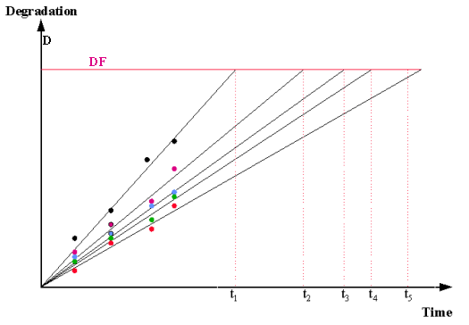
In many practical situations, \(D\) starts at 0 at time zero, and all the linear theoretical degradation lines start at the origin. This is the case when \(D\) is a "% change" parameter, or failure is defined as a change of a specified magnitude in a parameter, regardless of its starting value. Lines all starting at the origin simplify the analysis since we don't have to characterize the population starting value for \(D\), and the "distance" any unit "travels" to reach failure is always the constant \(DF\). For these situations, the degradation lines would look as follows.

Often, the degradation lines go through the origin - as when % change is the measurable parameter increasing to a failure level

It is also common to assume the effect of measurement error, when reading values of \(D\), has relatively little impact on the accuracy of model estimates.

Advantages of Modeling Based on Degradation Data

Modeling based on complete samples of measurement data, even with low stress cells, offers many advantages

1. Every degradation readout for every test unit contributes a data point. This leads to large amounts of useful data, even if there are very few failures.
2. You don't have to run tests long enough to obtain significant numbers of failures.
3. You can run low stress cells that are much closer to use conditions and obtain meaningful degradation data. The same cells would be a waste of time to run if failures were needed for modeling. Since these cells are more typical of use conditions, it makes sense to have them influence model parameters.
4. Simple plots of degradation versus time can be used to visually test the linear degradation assumption.

Drawbacks to Modeling Based on Degradation Data

Degradation may not proceed in a smooth, linear fashion towards what the customer calls "failure"

1. For many failure mechanisms, it is difficult or impossible to find a measurable parameter that degrades to a critical value in such a way that reaching that critical value is equivalent to what the customer calls a failure.
2. Degradation trends may vary erratically from unit to unit, with no apparent way to transform them into linear trends.
3. Sometimes degradation trends are reversible and a few units appear to "heal themselves" or get better. This kind of behavior does not follow typical assumptions and is difficult to model.
4. Measurement error may be significant and overwhelm small degradation trends, especially at low stresses.
5. Even when degradation trends behave according to assumptions and the chosen models fit well, the final results may not be consistent with an analysis based on actual failure data. This probably means that the failure mechanism depends on more than a simple continuous degradation process.

Because of the last listed drawback, it is a good idea to have at least one high-stress cell where enough real failures occur to do a standard life distribution model analysis. The parameter estimates obtained can be compared to the predictions from the degradation data analysis, as a "reality" check.

A Simple Method For Modeling Degradation Data

A simple approach is to extend each unit's degradation line until a projected "failure time" is obtained

1. As shown in the figures above, fit a line through each unit's degradation readings. This can be done by hand, but using a least squares regression program is better.
2. Take the equation of the fitted line, substitute \(DF\) for \(Y\) and solve for \(X\). This value of \(X\) is the "projected time of fail" for that unit.
3. Repeat for every unit in a stress cell until a complete sample of (projected) times of failure is obtained for the cell.
4. Use the failure times to compute life distribution parameter estimates for a cell. Under the fairly typical assumption of a lognormal model, this is very simple. Take natural logarithms of all failure times and treat the resulting data as a sample from a normal distribution. Compute the sample mean and the sample standard deviation. These are estimates of \(\mbox{ln } T_{50}\) and \(\sigma\), respectively, for the cell.
5. Assuming there are \(k\) cells with varying stress, fit an appropriate acceleration model using the cell \(\mbox{ln } T_{50}\) values, as described in the graphical estimation section. A single sigma estimate is obtained by taking the square root of the average of the cell \(\sigma^2\) estimates (assuming the same number of units each cell). If the cells have \(n_j\) units on test, where the \(n_j\) values are not all equal, use the pooled sum-of-squares estimate across all \(k\) cells calculated by

$$ \hat{\sigma}^2 = \frac{1}{\sum_{j=1}^k (n_j - 1)} \sum_{j=1}^k \sum_{i=1}^{n_j} \left( x_{ij} - \bar{x}_j \right)^2 \, . $$

A More Accurate Regression Approach For the Case When \(D\) = 0 at time 0 and the "Distance To Fail" \(DF\) is the Same for All Units

Models can be fit using all the degradation readings and linear regression

Let the degradation measurement for the \(i\)-th unit at the \(j\)-th readout time in the \(k\)-th stress cell be given by \(D_{ijk}\), and let the corresponding readout time be denoted by \(t_{jk}\). That readout gives a degradation rate (or slope) estimate of \(D_{ijk} / t_{jk}\). This follows from the linear assumption or:

(Rate of degradation) × (Time on test) = (Amount of degradation)

Based on that readout alone, an estimate of the natural logarithm of the time to fail for that unit is $$ y_{ijk} = \mbox{ln } DF - \left( \mbox{ln } D_{ijk} - \mbox{ln } t_{jk} \right) \, . $$

This follows from the basic formula connecting linear degradation with failure time

(rate of degradation) × (time of failure) = \(DF\)

by solving for (time of failure) and taking natural logarithms.

For an Arrhenius model analysis, with $$ t_f = A \cdot \mbox{exp}\left( \frac{\Delta H}{KT} \right) \, , $$ $$ y_{ijk} = a + b x_k \, , $$

with the \(x_k\) values equal to \(1/KT\). Here \(T\) is the temperature of the \(k\)-th cell, measured in Kelvin (273.16 + degrees Celsius) and \(K\) is Boltzmann's constant (8.617 × 10^-5 in eV/ unit Kelvin). Use a linear regression program to estimate \(a = \mbox{ln } A\) and \(b = \Delta H\). If we further assume \(t_f\) has a lognormal distribution, the mean square residual error from the regression fit is an estimate of \(\sigma^2\) (with \(\sigma\) the lognormal sigma).

One way to think about this model is as follows: each unit has a random rate \(R\) of degradation. Since \(t_f = DF/R\), it follows from a characterization property of the normal distribution that if is lognormal, then \(R\) must also have a lognormal distribution (assuming \(DF\) and \(R\) are independent). After we take logarithms, \(\mbox{ln } R\) has a normal distribution with a mean determined by the acceleration model parameters. The randomness in \(R\) comes from the variability in physical characteristics from unit to unit, due to material and processing differences.

Note: The estimate of sigma based on this simple graphical approach might tend to be too large because it includes an adder due to the measurement error that occurs when making the degradation readouts. This is generally assumed to have only a small impact.

Example: Arrhenius Degradation Analysis

An example using the regression approach to fit an Arrhenius model

A component has a critical parameter that studies show degrades linearly over time at a rate that varies with operating temperature. A component failure based on this parameter occurs when the parameter value changes by 30 % or more. Fifteen components were tested under 3 different temperature conditions (5 at 65 °C, 5 at 85 °C and the last 5 at 105 °C). Degradation percent values were read out at 200, 500 and 1000 hours. The readings are given by unit in the following three temperature cell tables.

65 °C

200 hr	500 hr	1000 hr
Unit 1      0.87	1.48	2.81
Unit 2      0.33	0.96	2.13
Unit 3      0.94	2.91	5.67
Unit 4      0.72	1.98	4.28
Unit 5      0.66	0.99	2.14

 85 °C

200 hr	500 hr	1000 hr
Unit 1      1.41	2.47	5.71
Unit 2      3.61	8.99	17.69
Unit 3      2.13	5.72	11.54
Unit 4      4.36	9.82	19.55
Unit 5      6.91	17.37	34.84

 105 °C

200 hr	500 hr	1000 hr
Unit 1      24.58	62.02	124.10
Unit 2       9.73	24.07	48.06
Unit 3       4.74	11.53	23.72
Unit 4      23.61	58.21	117.20
Unit 5      10.90	27.85	54.97

Note that one unit failed in the 85 °C cell and four units failed in the 105 °C cell. Because there were so few failures, it would be impossible to fit a life distribution model in any cell but the 105 °C cell, and therefore no acceleration model can be fit using failure data. We will fit an Arrhenius/lognormal model, using the degradation data.

Solution:

Fit the model to the degradation data

From the above tables, first create a variable (\(DEG\)) with 45 degradation values starting with the first row in the first table and proceeding to the last row in the last table. Next, create a temperature variable (\(TEMP\)) that has 15 repetitions of 65, followed by 15 repetitions of 85 and then 15 repetitions of 105. Finally, create a time variable (\(TIME\)) that corresponds to readout times.

Fit the Arrhenius/lognormal equation, \(y_{ijk} = a + bx_{ijk}\), where $$ y_{ijk} = \mbox{ln } 30 - \left( \mbox{ln } DEG - \mbox{ln } TIME \right) $$ and $$ x_{ijk} = \frac{100000}{8.617(TEMP + 273.16)} \, . $$

The linear regression results are the following.

   Parameter     Estimate   Stan. Dev   t Value
   ---------     --------   ---------   -------
   a            -18.94337    1.83343     -10.33 
   b              0.81877    0.05641      14.52 
 
   Residual standard deviation = 0.5611 
   Residual degrees of freedom = 45

The Arrhenius model parameter estimates are: \(\mbox{ln } A\) = -18.94; \(\Delta H\) = 0.82. An estimate of the lognormal sigma is \(\sigma\) = 0.56.

The analyses in this section can can be implemented using both Dataplot code and R code.