1.3. EDA Techniques
1.3.3. Graphical Techniques: Alphabetic
1.3.3.15. Lag Plot
1.3.3.15.4. |
Lag Plot: Sinusoidal Models and Outliers |

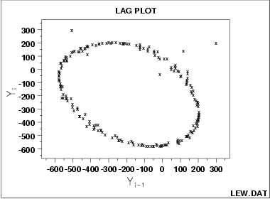
- The data come from an underlying single-cycle sinusoidal model.
- The data contain three outliers.
-
\[ Y_{i} = A_0 + E_{i} \]
- the sample mean would be biased and meaningless;
- the confidence limits would be meaningless and optimistically small.
-
\[ Y_{i} = C + \alpha\sin{(2\pi\omega t_{i} + \phi)} + E_{i} \]
The lag plot is also of value in outlier detection. Note in the above plot that there appears to be 4 points lying off the ellipse. However, in a lag plot, each point in the original data set Y shows up twice in the lag plot--once as Yi and once as Yi-1. Hence the outlier in the upper left at Yi = 300 is the same raw data value that appears on the far right at Yi-1 = 300. Thus (-500,300) and (300,200) are due to the same outlier, namely the 158th data point: 300. The correct value for this 158th point should be approximately -300 and so it appears that a sign got dropped in the data collection. The other two points lying off the ellipse, at roughly (100,100) and at (0,-50), are caused by two faulty data values: the third data point of -15 should be about +125 and the fourth data point of +141 should be about -50, respectively. Hence the 4 apparent lag plot outliers are traceable to 3 actual outliers in the original run sequence: at points 4 (-15), 5 (141) and 158 (300). In retrospect, only one of these (point 158 (= 300)) is an obvious outlier in the run sequence plot.
- Do a spectral plot to obtain an initial estimate of the
frequency of the underlying cycle. This will be helpful
as a starting value for the subsequent non-linear fitting.
- Omit the outliers.
- Carry out a non-linear fit of the model to the 197 points.
-
\[ Y_{i} = C + \alpha\sin{(2\pi\omega t_{i} + \phi)} + E_{i} \]

