1. Exploratory Data Analysis
1.4. EDA Case Studies
1.4.2. Case Studies
1.4.2.3. Random Walk

1.4.2.3.4.

Validate New Model

Plot Predicted with Original Data

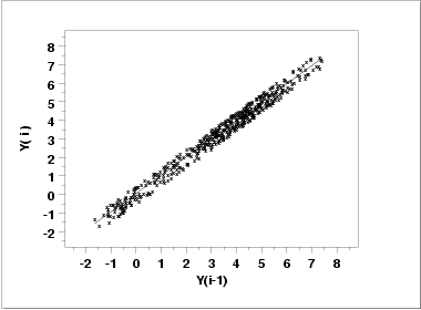
The first step in verifying the model is to plot the predicted values from the fit with the original data.

This plot indicates a reasonably good fit.

Test Underlying Assumptions on the Residuals

In addition to the plot of the predicted values, the residual standard deviation from the fit also indicates a significant improvement for the model. The next step is to validate the underlying assumptions for the error component, or residuals, from this model.

4-Plot of Residuals

Interpretation

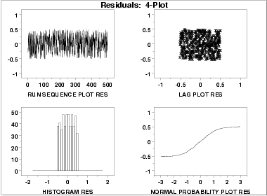
The assumptions are addressed by the graphics shown above:

1. The run sequence plot (upper left) indicates no significant shifts in location or scale over time.

2. The lag plot (upper right) exhibits a random appearance.

3. The histogram shows a relatively flat appearance. This indicates that a uniform probability distribution may be an appropriate model for the error component (or residuals).

4. The normal probability plot clearly shows that the normal distribution is not an appropriate model for the error component.

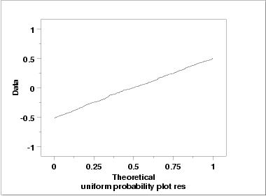
A uniform probability plot can be used to further test the suggestion that a uniform distribution might be a good model for the error component.

Uniform Probability Plot of Residuals

Since the uniform probability plot is nearly linear, this verifies that a uniform distribution is a good model for the error component.

Conclusions

Since the residuals from our model satisfy the underlying assumptions, we conlude that

\( Y_{i} = 0.0502 + 0.987*Y_{i-1} + E_{i} \)

where the E_i follow a uniform distribution is a good model for this data set. We could simplify this model to

\( Y_{i} = 1.0*Y_{i-1} + E_{i} \)

This has the advantage of simplicity (the current point is simply the previous point plus a uniformly distributed error term).

Using Scientific and Engineering Knowledge

In this case, the above model makes sense based on our definition of the random walk. That is, a random walk is the cumulative sum of uniformly distributed data points. It makes sense that modeling the current point as the previous point plus a uniformly distributed error term is about as good as we can do. Although this case is a bit artificial in that we knew how the data were constructed, it is common and desirable to use scientific and engineering knowledge of the process that generated the data in formulating and testing models for the data. Quite often, several competing models will produce nearly equivalent mathematical results. In this case, selecting the model that best approximates the scientific understanding of the process is a reasonable choice.

Time Series Model

This model is an example of a time series model. More extensive discussion of time series is given in the Process Monitoring chapter.