2. Measurement Process Characterization
2.6. Case studies
2.6.5. Uncertainty analysis for extinguishing fire

2.6.5.2.

Create a calibration curve for the rotameter

The primary topic of this case study is on computing uncertainties. If you want to skip the model fitting stage, you can choose to view the final model only or go directly to the computation of the predicted values and the uncertainties of the predicted values.

Plot of the Data

The first step in the analysis is to create a calibration curve for the rotameter. This is accomplished by fitting a curve to the data points.

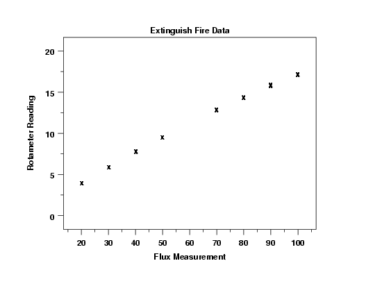
We plot the data in order to determine an appropriate model.

This plot indicates that a linear model might be approriate. It also shows that the replicated points show very little deviation. That is, for each X value it appears that there is a single point when in fact there are 10 points.

Standard Deviation Plot

We can use a standard deviation plot to get a better view of the variation in the data.

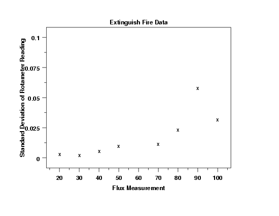
Although the standard deviations are quite small, the standard deviation plot shows the standard deviation increasing as the value of flux increases. The increase is particularly notable at flux equal 90.

Plot with Group Means Subtracted

It would be interesting to know if this increasing spread is due to a few outliers or is indicative of a pattern of increasing variation as the value of flux increases. We can show this by subtracting the group mean of the data values at each value of flux.

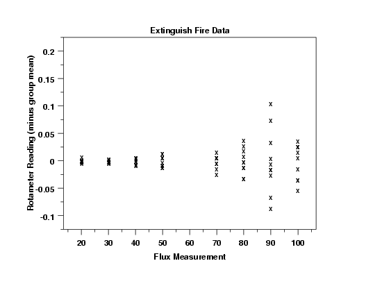
This plot shows clearly that the variation is increasing as the value of flux increases. This means that we may need to use weighting or transformations in developing the calibration curve.

Linear Fit

The initial plot indicated that a linear model might be adequate. Dataplot generated the following output for a linear fit (the output has been edited slightly for display).

  
LEAST SQUARES POLYNOMIAL FIT
SAMPLE SIZE N       =       80
DEGREE              =        1
REPLICATION CASE
REPLICATION STANDARD DEVIATION =     0.2554919757D-01
REPLICATION DEGREES OF FREEDOM =          72
NUMBER OF DISTINCT SUBSETS     =           8
  
  
        PARAMETER ESTIMATES           (APPROX. ST. DEV.)    T VALUE
 1  A0                   1.09419       (0.6796E-01)          16.
 2  A1                  0.164900       (0.1030E-02)         0.16E+03
  
RESIDUAL    STANDARD DEVIATION =         0.2523804009
RESIDUAL    DEGREES OF FREEDOM =          78
REPLICATION STANDARD DEVIATION =         0.0255491976
REPLICATION DEGREES OF FREEDOM =          72
LACK OF FIT F RATIO =    1256.5281 = THE 100.0000% POINT OF THE
F DISTRIBUTION WITH      6 AND     72 DEGREES OF FREEDOM
  

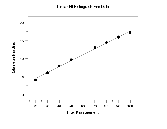
The linear fit generated the model

This model has a residual standard deviation of 0.254.

Plot of Predicted Values with Raw Data

To assess the validity of the fit, we plot the predicted values with the raw data.

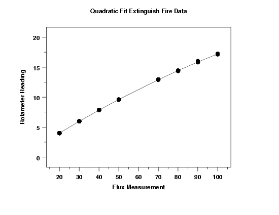
This plot indicates a good fit.

4-Plot of Residuals

The next step in the model validation is a residual analysis to test the model assumptions. We generate a 4-plot of the residuals to do this.

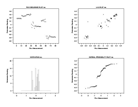
This 4-plot reveals serious violations of the regression assumptions. Specifically, the run sequence plot in the upper left corner shows a non-random pattern and it shows a violation of the assumption of constant location for the residuals. The lag plot in the upper right corner shows that the residuals have a strong autocorrelation, which violates the assumption of randomness for the residuals. When the randomness assumption is violated, the distributional plots (the histogram in the lower left corner and the normal probability plot in the lower right corner) are not meaningful.

Quadratic Fit

To address these assumption violations, we next fit a quadratic model.

  
LEAST SQUARES POLYNOMIAL FIT
SAMPLE SIZE N       =       80
DEGREE              =        2
REPLICATION CASE
REPLICATION STANDARD DEVIATION =     0.2554919757D-01
REPLICATION DEGREES OF FREEDOM =          72
NUMBER OF DISTINCT SUBSETS     =           8
  
  
        PARAMETER ESTIMATES           (APPROX. ST. DEV.)    T VALUE
 1  A0                 -0.144687       (0.2165E-01)         -6.7
 2  A1                  0.217063       (0.8339E-03)         0.26E+03
 3  A2                 -0.434694E-03   (0.6847E-05)         -63.
  
RESIDUAL    STANDARD DEVIATION =         0.0347798578
RESIDUAL    DEGREES OF FREEDOM =          77
REPLICATION STANDARD DEVIATION =         0.0255491976
REPLICATION DEGREES OF FREEDOM =          72
LACK OF FIT F RATIO =      14.1379 = THE 100.0000% POINT OF THE
F DISTRIBUTION WITH      5 AND     72 DEGREES OF FREEDOM
  

The fitted quadratic model is

The residual standard deviation is now 0.035. This is nearly a factor of 10 reduction.

Plot of Predicted Values with Raw Data

To assess the model, we generate the plot of the predicted values with the raw data.

4-Plot of Residuals

We again use the 4-plot to do a residual analysis.

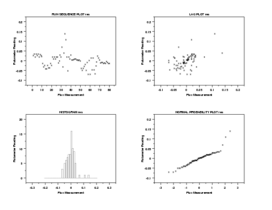
This 4-plot does not show major violations of the regression assumptions. The run sequence plot of the residuals in the upper left corner indicates constant location and scale for the residuals. The lag plot in the upper right corner does not show significant autocorrelation for the residuals. The histogram and normal probability plot indicate that the residuals are reasonably approximated by a normal distribution.

Outliers

Even though the 4-plot above showed a reasonable fit, all four of these plots indicate a few outliers. These are due to the increasing standard deviation as the value of flux increases.

There are several approaches we can take towards addressing the outliers in the residual plots.

• We can accept the quadratic fit as an adequate fit.
• We can use weighting where the weights are proportional to the variance.
• We can use bisquare weighting of the residuals.
• We can delete specific points as outliers.

Final Model

For this particular data set, there is little practical difference in the fitted quadratic model regardless of which approach was used. We have taken the trouble to show the different approaches because each of these approaches, or some combination of these approaches, may be useful for other data sets.

For this case study, we will use the quadratic model based on deleting two outliers.