4. Process Modeling
4.1. Introduction to Process Modeling

4.1.1.

What is process modeling?

Basic Definition

Process modeling is the concise description of the total variation in one quantity, y, by partitioning it into

1. a deterministic component given by a mathematical function of one or more other quantities, x₁, x₂, ... , plus
   
   
2. a random component that follows a particular probability distribution.

Example

For example, the total variation of the measured pressure of a fixed amount of a gas in a tank can be described by partitioning the variability into its deterministic part, which is a function of the temperature of the gas, plus some left-over random error. Charles' Law states that the pressure of a gas is proportional to its temperature under the conditions described here, and in this case most of the variation will be deterministic. However, due to measurement error in the pressure gauge, the relationship will not be purely deterministic. The random errors cannot be characterized individually, but will follow some probability distribution that will describe the relative frequencies of occurrence of different-sized errors. (The reader can download the pressure/temperature data as a text file.)

Graphical Interpretation

Using the example above, the definition of process modeling can be graphically depicted like this:

Click Figure for Full-Sized Copy

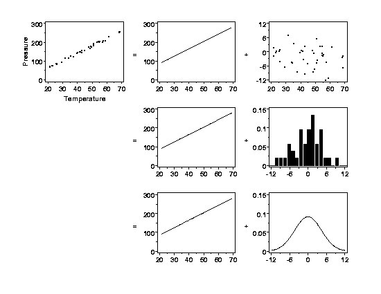
The top left plot in the figure shows pressure data that vary deterministically with temperature except for a small amount of random error. The relationship between pressure and temperature is a straight line, but not a perfect straight line. The top row plots on the right-hand side of the equals sign show a partitioning of the data into a perfect straight line and the remaining "unexplained" random variation in the data (note the different vertical scales of these plots). The plots in the middle row of the figure show the deterministic structure in the data again and a histogram of the random variation. The histogram shows the relative frequencies of observing different-sized random errors. The bottom row of the figure shows how the relative frequencies of the random errors can be summarized by a (normal) probability distribution.

An Example from a More Complex Process

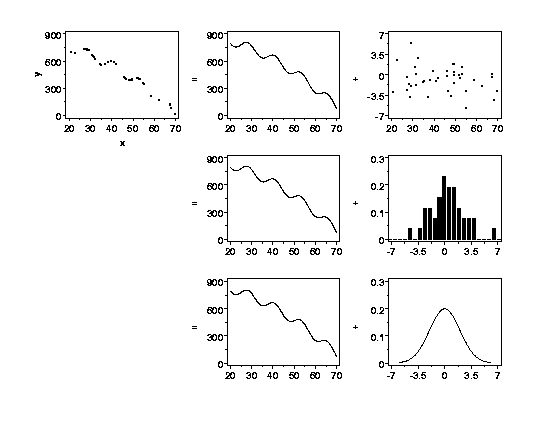
Of course, the straight-line example is one of the simplest functions used for process modeling. Another example is shown below. The concept is identical to the straight-line example, but the structure in the data is more complex. The variation in y is partitioned into a deterministic part, which is a function of another variable, x, plus some left-over random variation. (Again note the difference in the vertical axis scales of the two plots in the top right of the figure.) A probability distribution describes the leftover random variation.

An Example with Multiple Explanatory Variables

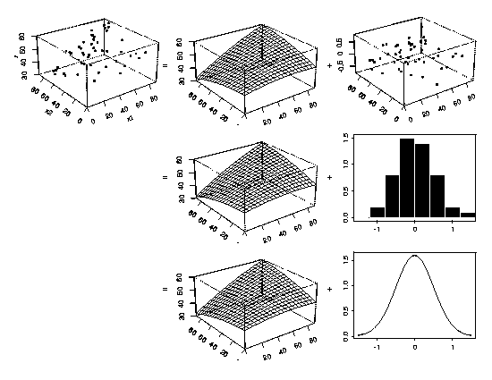
The examples of process modeling shown above have only one explanatory variable but the concept easily extends to cases with more than one explanatory variable. The three-dimensional perspective plots below show an example with two explanatory variables. Examples with three or more explanatory variables are exactly analogous, but are difficult to show graphically.