4. Process Modeling
4.6. Case Studies in Process Modeling
4.6.2. Alaska Pipeline

4.6.2.3.

Initial Linear Fit

Linear Fit Results

Based on the initial plot of the data, we first fit a straight-line model to the data.

Parameter     Estimate    Stan. Dev    t Value
B0             4.99368      1.12566       4.44
B1             0.73111      0.02455      29.78
  
Residual standard deviation = 6.08092
Residual degrees of freedom = 105

Lack-of-fit F statistic              = 0.9857
Lack-of-fit critical value, F0.05,76,29 = 1.73

The intercept parameter is estimated to be 4.99368 and the slope parameter is estimated to be 0.73111. Both parameters are statistically significant.

6-Plot for Model Validation

When there is a single independent variable, the 6-plot provides a convenient method for initial model validation.

The basic assumptions for regression models are that the errors are random observations from a normal distribution with mean of zero and constant standard deviation (or variance).

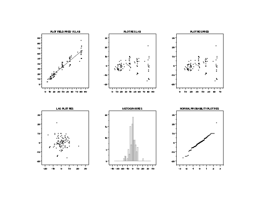
The plots on the first row show that the residuals have increasing variance as the value of the independent variable (lab) increases in value. This indicates that the assumption of constant standard deviation, or homogeneity of variances, is violated.

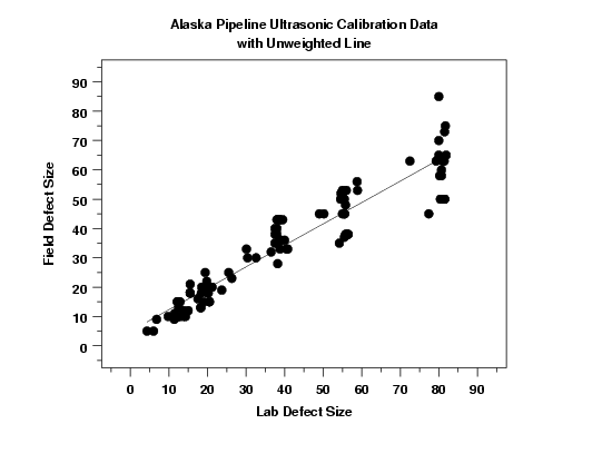
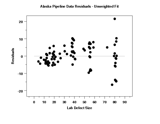
In order to see this more clearly, we will generate full- size plots of the predicted values with the data and the residuals against the independent variable.

Plot of Predicted Values with Original Data

This plot shows more clearly that the assumption of homogeneous variances for the errors may be violated.

Plot of Residual Values Against Independent Variable

This plot also shows more clearly that the assumption of homogeneous variances is violated. This assumption, along with the assumption of constant location, are typically easiest to see on this plot.

Non-Homogeneous Variances

Because the last plot shows that the variances may differ more that slightly, we will address this issue by transforming the data or using weighted least squares.