5.
Process Improvement
5.5.
Advanced topics
5.5.5.
|
How can I account for nested variation (restricted randomization)?
|
|
|
Nested data structures are common and lead to many sources of
variability
|
Many processes have more than one source of variation in them. In order
to reduce variation in processes, these multiple sources must be
understood, and that often leads to the concept of nested or
hierarchical data structures. For example, in the semiconductor
industry, a batch process may operate on several wafers at a time
(wafers are said to be nested within batch). Understanding
the input variables that control variation among those wafers, as well
as understanding the variation across each wafer in a run, is an
important part of the strategy for minimizing the total variation in
the system.
|
|
Example of nested data
|
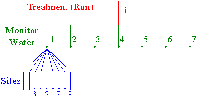
Figure 5.15 below represents a batch process that uses 7 monitor
wafers in each run. The plan further calls for measuring response on
each wafer at each of 9 sites. The organization of the sampling plan
has a hierarchical or nested structure: the batch run is the topmost
level, the second level is an individual wafer, and the third level is
the site on the wafer.
The total amount of data generated per batch run will be 7*9 = 63 data
points. One approach to analyzing these data would be to compute the
mean of all these points as well as their standard deviation and use
those results as responses for each run.
|
|
Diagram illustrating the example
|

FIGURE 5.15: Hierarchical Data Structure Example
|
|
Sites nested within wafers and wafers are nested within runs
|
Analyzing the data as suggested above is not absolutely incorrect,
but doing so loses information that one might otherwise obtain. For
example, site 1 on wafer 1 is physically different from site 1 on
wafer 2 or on any other wafer. The same is true for any of the sites
on any of the wafers. Similarly, wafer 1 in run 1 is physically
different from wafer 1 in run 2, and so on. To describe this situation
one says that sites are nested within wafers while wafers
are nested within runs.
|
|
Nesting places restrictions on the randomization
|
As a consequence of this nesting, there are restrictions on the
randomization that can occur in the experiment. This kind of
restricted randomization always produces nested sources of variation.
Examples of nested variation or restricted randomization discussed on
this page are split-plot and
strip-plot designs.
|
Wafer-to-
wafer and site-to-site variations are often "noise factors"
in an experiment
|
The objective of an experiment with the type of sampling plan
described in Figure 5.15 is generally to reduce the variability due
to sites on the wafers and wafers within runs (or batches) in the
process. The sites on the wafers and the wafers within a batch become
sources of unwanted variation and an investigator seeks to make the
system robust to those sources -- in other words, one could
treat wafers and sites as noise factors in such an experiment.
|
|
Treating wafers and sites as random effects allows calculation of
variance estimates
|
Because the wafers and the sites represent unwanted sources of variation
and because one of the objectives is to reduce the process sensitivity
to these sources of variation, treating wafers and sites as random
effects in the analysis of the data is a reasonable approach. In other
words, nested variation is often another way of saying nested random
effects or nested sources of noise. If the factors "wafers" and
"sites", are treated as random effects, then it is possible to estimate
a variance component due to each source of variation through analysis
of variance techniques. Once estimates of the variance components
have been obtained, an investigator is then able to determine the
largest source of variation in the process under experimentation, and
also determine the magnitudes of the other sources of variation in
relation to the largest source.
|
|
Nested random effects same as nested variation
|
If an experiment or process has nested variation, the experiment or
process has multiple sources of random error that affect its output.
Having nested random effects in a model is the same thing as having
nested variation in a model.
|
|
|
Split-Plot Designs
|
|
Split-plot designs often arise when some factors are "hard to vary"
or when batch processes are run
|
Split-plot designs result when a particular type of restricted
randomization has occurred during the experiment. A simple factorial
experiment can result in a split-plot type of design because of the
way the experiment was actually executed.
In many industrial experiments, three situations often occur:
- some of the factors of interest may be 'hard to vary' while
the remaining factors are easy to vary. As a result, the order
in which the treatment combinations for the experiment are run
is determined by the ordering of these 'hard-to-vary'
factors
- experimental units are processed together as a batch for one or
more of the factors in a particular treatment combination
- experimental units are processed individually, one right after
the other, for the same treatment combination without resetting
the factor settings for that treatment combination.
|
|
A split-plot experiment example
|
An experiment run under one of the above three situations usually
results in a split-plot type of design. Consider an experiment to
examine electroplating of aluminum (non-aqueous) on copper strips. The
three factors of interest are: current (A); solution temperature (T);
and the solution concentration of the plating agent (S). Plating rate
is the measured response. There are a total of 16 copper strips
available for the experiment. The treatment combinations to be run
(orthogonally scaled) are listed below in standard order (i.e., they
have not been randomized):
|
|
Table showing the design matrix
|
TABLE 5.6: Orthogonally Scaled Treatment Combinations
from a 23 Full Factorial
|
Current
|
Temperature
|
Concentration
|
|
|
-1
|
-1
|
-1
|
|
-1
|
-1
|
+1
|
|
-1
|
+1
|
-1
|
|
-1
|
+1
|
+1
|
|
+1
|
-1
|
-1
|
|
+1
|
-1
|
+1
|
|
+1
|
+1
|
-1
|
|
+1
|
+1
|
+1
|
|
|
Concentration is hard to vary, so minimize the number of times
it is changed
|
Consider running the experiment under the first condition listed above,
with the factor solution concentration of the plating agent (S) being
hard to vary. Since this factor is hard to vary, the experimenter would
like to randomize the treatment combinations so that the solution
concentration factor has a minimal number of changes. In other words,
the randomization of the treatment runs is restricted somewhat by the
level of the solution concentration factor.
|
|
Randomize so that all runs for one level of concentration are
run first
|
As a result, the treatment combinations might be randomized such that
those treatment runs corresponding to one level of the concentration
(-1) are run first. Each copper strip is individually plated, meaning
only one strip at a time is placed in the solution for a given
treatment combination. Once the four runs at the low level of
solution concentration have been completed, the solution is changed
to the high level of concentration (1), and the remaining four runs of
the experiment are performed (where again, each strip is individually
plated).
|
|
Performing replications
|
Once one complete replicate of the experiment has been completed, a
second replicate is performed with a set of four copper strips
processed for a given level of solution concentration before changing
the concentration and processing the remaining four strips. Note
that the levels for the remaining two factors can still be randomized.
In addition, the level of concentration that is run first in the
replication runs can also be randomized.
|
|
Whole plot and subplot factors
|
Running the experiment in this way results in a split-plot design.
Solution concentration is known as the whole plot factor and the
subplot factors are the current and the solution temperature.
|
|
Definition of experimental units and whole plot and subplot factors
for this experiment
|
A split-plot design has more than one size
experimental unit.
In this experiment, one size experimental unit is an individual
copper strip. The treatments or factors that were applied to the
individual strips are solution temperature and current (these factors
were changed each time a new strip was placed in the solution). The
other or larger size experimental unit is a set of four copper strips.
The treatment or factor that was applied to a set of four strips is
solution concentration (this factor was changed after four strips were
processed). The smaller size experimental unit is referred to as the
subplot experimental unit, while the larger experimental unit is
referred to as the whole plot unit.
|
|
Each size of experimental unit leads to an error term in the model
for the experiment
|
There are 16 subplot experimental units for this experiment. Solution
temperature and current are the subplot factors in this experiment.
There are four whole-plot experimental units in this experiment.
Solution concentration is the whole-plot factor in this experiment.
Since there are two sizes of experimental units, there are two error
terms in the model, one that corresponds to the whole-plot error
or whole-plot experimental unit and one that corresponds to the subplot
error or subplot experimental unit.
|
|
Partial ANOVA table
|
The ANOVA table for this experiment would look, in part, as follows:
Source                                   DF

Replication                               1
Concentration                             1
Error (Whole plot) = Rep*Conc             1
Temperature                               1
Rep*Temp                                  1
Current                                   1
Rep*Current                               1
Temp*Conc                                 1
Rep*Temp*Conc                             1
Temp*Current                              1
Rep*Temp*Current                          1
Current*Conc                              1
Rep*Current*Conc                          1
Temp*Current*Conc                         1
Error (Subplot) =Rep*Temp*Current*Conc    1
The first three sources are from the whole-plot level, while the next
12 are from the subplot portion. A
normal probability plot
of the 12 subplot term estimates could be used to look for
significant terms.
|
|
A batch process leads to a different experiment - also a
strip-plot
|
Consider running the experiment under the second condition listed above
(i.e., a batch process) for which four copper strips are placed in the
solution at one time. A specified level of current can be applied to an
individual strip within the solution. The same 16 treatment combinations
(a replicated 23 factorial) are run as were run under the
first scenario. However, the way in which the experiment is performed
would be different. There are four treatment combinations of solution
temperature and solution concentration: (-1, -1), (-1, 1), (1, -1),
(1, 1). The experimenter randomly chooses one of these four treatments
to set up first. Four copper strips are placed in the solution. Two of
the four strips are randomly assigned to the low current level. The
remaining two strips are assigned to the high current level. The
plating is performed and the response is measured. A second treatment
combination of temperature and concentration is chosen and the same
procedure is followed. This is done for all four
temperature / concentration combinations.
|
|
This also a split-plot design
|
Running the experiment in this way also results in a split-plot design
in which the whole-plot factors are now solution concentration and
solution temperature, and the subplot factor is current.
|
|
Defining experimental units
|
In this experiment, one size experimental unit is again an individual
copper strip. The treatment or factor that was applied to the individual
strips is current (this factor was changed each time for a different
strip within the solution). The other or larger size experimental unit
is again a set of four copper strips. The treatments or factors that
were applied to a set of four strips are solution concentration and
solution temperature (these factors were changed after four strips
were processed).
|
|
Subplot experimental unit
|
The smaller size experimental unit is again referred to as the subplot
experimental unit. There are 16 subplot experimental units for this
experiment. Current is the subplot factor in this experiment.
|
|
Whole-plot experimental unit
|
The larger-size experimental unit is the whole-plot experimental unit.
There are four whole plot experimental units in this experiment and
solution concentration and solution temperature are the whole plot
factors in this experiment.
|
|
Two error terms in the model
|
There are two sizes of experimental units and there are two
error terms in the model: one that corresponds to the whole-plot
error or whole-plot experimental unit, and one that corresponds to
the subplot error or subplot experimental unit.
|
|
Partial ANOVA table
|
The ANOVA for this experiment looks, in part, as follows:
Source                             DF

Concentration                       1
Temperature                         1
Error (Whole plot) = Conc*Temp      1

Current                             1
Conc*Current                        1
Temp*Current                        1
Conc*Temp*Current                   1
Error (Subplot)                     8
The first three sources come from the whole-plot level and the next
5 come from the subplot level. Since there are 8 degrees of freedom for
the subplot error term, this MSE can be used to test each effect that
involves current.
|
|
Running the experiment under the third scenario
|
Consider running the experiment under the third scenario listed above.
There is only one copper strip in the solution at one time. However,
two strips, one at the low current and one at the high current, are
processed one right after the other under the same temperature and
concentration setting. Once two strips have been processed, the
concentration is changed and the temperature is reset to another
combination. Two strips are again processed, one after the other, under
this temperature and concentration setting. This process is continued
until all 16 copper strips have been processed.
|
|
This also a split-plot design
|
Running the experiment in this way also results in a split-plot design
in which the whole-plot factors are again solution concentration and
solution temperature and the subplot factor is current. In this
experiment, one size experimental unit is an individual copper strip.
The treatment or factor that was applied to the individual strips is
current (this factor was changed each time for a different strip within
the solution). The other or larger-size experimental unit is a set of
two copper strips. The treatments or factors that were applied to a
pair of two strips are solution concentration and solution temperature
(these factors were changed after two strips were processed). The
smaller size experimental unit is referred to as the subplot
experimental unit.
|
|
Current is the subplot factor and temperature and concentration are
the whole plot factors
|
There are 16 subplot experimental units for this experiment. Current
is the subplot factor in the experiment. There are eight whole-plot
experimental units in this experiment. Solution concentration and
solution temperature are the whole plot factors. There are two error
terms in the model, one that corresponds to the whole-plot error or
whole-plot experimental unit, and one that corresponds to the subplot
error or subplot experimental unit.
|
|
Partial ANOVA table
|
The ANOVA for this (third) approach is, in part, as follows:
Source                          DF

Concentration                  1
Temperature                    1
Conc*Temp                      1
Error (Whole plot)             4

Current                        1
Conc*Current                   1
Temp*Current                   1
Conc*Temp*Current              1
Error (Subplot)                4
The first four terms come from the whole-plot analysis and the next
5 terms come from the subplot analysis. Note that we have separate error
terms for both the whole plot and the subplot effects, each based on 4
degrees of freedom.
|
|
Primary distinction of split-plot designs is that they have more than
one experimental unit size (and therefore more than one error term)
|
As can be seen from these three scenarios, one of the major
differences in split-plot designs versus simple factorial designs is
the number of different sizes of experimental units in the experiment.
Split-plot designs have more than one size experimental unit, i.e.,
more than one error term. Since these designs involve different sizes
of experimental units and different variances, the standard errors of
the various mean comparisons involve one or more of the variances.
Specifying the appropriate model for a split-plot design involves
being able to identify each size of experimental unit. The way an
experimental unit is defined relative to the design structure (for
example, a completely randomized design versus a randomized complete
block design) and the treatment structure (for example, a full
23 factorial, a resolution V half fraction, a two-way
treatment structure with a control group, etc.). As a result of having
greater than one size experimental unit, the appropriate model used
to analyze split-plot designs is a mixed model.
|
|
Using wrong model can lead to invalid conclusions
|
If the data from an experiment are analyzed with only one error term
used in the model, misleading and invalid conclusions can be drawn
from the results. For a more detailed discussion of these designs
and the appropriate analysis procedures, see
Milliken, Analysis
of Messy Data, Vol. 1.
|
|
|
Strip-Plot Designs
|
|
Strip-plot desgins often result from experiments that are conducted
over two or more process steps
|
Similar to a split-plot design, a strip-plot design can result when
some type of restricted randomization has occurred during the
experiment. A simple factorial design can result in a strip-plot
design depending on how the experiment was conducted. Strip-plot
designs often result from experiments that are conducted over two or
more process steps in which each process step is a batch process, i.e.,
completing each treatment combination of the experiment requires more
than one processing step with experimental units processed together
at each process step. As in the split-plot design, strip-plot designs
result when the randomization in the experiment has been restricted
in some way. As a result of the restricted randomization that occurs
in strip-plot designs, there are multiple sizes of experimental
units. Therefore, there are different error terms or different error
variances that are used to test the factors of interest in the design.
A traditional strip-plot design has three sizes of experimental units.
|
|
Example with two steps and three factor variables
|
Consider the following example from the semiconductor industry. An
experiment requires an implant step and an anneal step. At both the
anneal and the implant steps there are three factors to test. The
implant process accommodates 12 wafers in a batch, and implanting a
single wafer under a specified set of conditions is not practical nor
does doing so represent economical use of the implanter. The anneal
furnace can handle up to 100 wafers.
|
|
Explanation of the diagram that illustrates the design structure
of the example
|
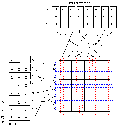
The figure below shows the design structure for how the experiment was
run. The rectangles at the top of the diagram represent the settings
for a two-level factorial design for the three factors in the implant
step (A, B, C). Similarly, the rectangles at the lower left of the
diagram represent a two-level factorial design for the three factors
in the anneal step (D, E, F).
The arrows connecting each set of rectangles to the grid in the center
of the diagram represent a randomization of trials in the experiment.
The horizontal elements in the grid represent the experimental units
for the anneal factors. The vertical elements in the grid represent
the experimental units for the implant factors. The intersection of
the vertical and horizontal elements represents the experimental units
for the interaction effects between the implant factors and the anneal
factors. Therefore, this experiment contains three sizes of
experimental units, each of which has a unique error term for
estimating the significance of effects.
|
|
Diagram of the split-plot design
|

FIGURE 5.16: Diagram of a strip-plot design involving two
process steps with three factors in each step
|
|
Physical meaning of the experimental units
|
To put actual physical meaning to each of the experimental units in
the above example, consider each cell in the grid as an individual
wafer. A batch of eight wafers goes through the implant step first.
According to the figure, treatment combination #3 in factors A, B,
and C is the first implant treatment run. This implant treatment is
applied to all eight wafers at once. Once the first implant treatment
is finished, another set of eight wafers is implanted with treatment
combination #5 of factors A, B, and C. This continues until the last
batch of eight wafers is implanted with treatment combination #6 of
factors A, B, and C. Once all of the eight treatment combinations of
the implant factors have been run, the anneal step starts. The first
anneal treatment combination to be run is treatment combination
#5 of factors D, E, and F. This anneal treatment combination is applied
to a set of eight wafers, with each of these eight wafers coming from
one of the eight implant treatment combinations. After this first batch
of wafers has been annealed, the second anneal treatment is applied
to a second batch of eight wafers, with these eight wafers coming from
one each of the eight implant treatment combinations. This is continued
until the last batch of eight wafers has been implanted with a
particular combination of factors D, E, and F.
|
|
Three sizes of experimental units
|
Running the experiment in this way results in a strip-plot design with
three sizes of experimental units. A set of eight wafers that are
implanted together is the experimental unit for the implant factors A,
B, and C and for all of their interactions. There are eight
experimental units for the implant factors. A different set of eight
wafers are annealed together. This different set of eight wafers is
the second size experimental unit and is the experimental unit for the
anneal factors D, E, and F and for all of their interactions. The third
size experimental unit is a single wafer. This is the experimental
unit for all of the interaction effects between the implant factors
and the anneal factors.
|
|
Replication
|
Actually, the above figure of the strip-plot design represents one
block or one replicate of this experiment. If the experiment contains
no replication and the model for the implant contains only the main
effects and two-factor interactions, the three-factor interaction
term A*B*C (1 degree of freedom) provides the error term for the
estimation of effects within the implant experimental unit. Invoking a
similar model for the anneal experimental unit produces the
three-factor interaction term D*E*F for the error term (1 degree of
freedom) for effects within the anneal experimental unit.
|
|
Further information
|
For more details about strip-plot designs, see
Milliken and
Johnson (1987) or
Miller (1997).
|


