Familiarity with the basic concepts and techniques from probability theory and
mathematical statistics can best be gained by studying suitable textbooks and
exercising those concepts and techniques by solving instructive problems.
The books by DeGroot and Schervish [2011], Hoel et al. [1971a], Hoel
et al. [1971b], Feller [1968], Lindley [1965a], and Lindley [1965b] are highly
recommended for this purpose and appropriate for readers who will have studied
mathematical calculus in university courses for science and engineering
majors.
This document aims to provide an overview of some of these concepts and
techniques that have proven useful in applications to the characterization,
propagation, and interpretation of measurement uncertainty as described, for
example, by Morgan and Henrion [1992] and Taylor and Kuyatt [1994], and in
guidance documents produced by international organizations, including the Guideto the expression of uncertainty in measurement (GUM) [Joint Committee for
Guides in Metrology, 2008a] and its supplements [Joint Committee for Guides in
Metrology, 2008b]. However, the examples do not all necessarily show a direct
connection to measurement science.
Our basic premises are that probability is best suited to express uncertainty
quantitatively, and that Bayesian statistical methods afford the best means to
exploit information about quantities of interest that originates from multiple
sources, including empirical data gathered for the purpose, and preexisting expert
knowledge.
Although there is nothing particularly controversial about the calculus of
probability or about the mathematical methods of statistics, both the meaning of
probability and the interpretation of the products of statistical inference continue
to be subjects of debate.
This debate is meta-probabilistic and meta-statistical, in the same sense as
metaphysics employs methods different from the methods of physics to study the
world. In fact, the debate is liveliest and most scholarly among professional
philosophers [Fitelson, 2007]. However, probabilists and statisticians often
participate in it when they take off their professional hats and become
philosophers [Neyman, 1977], as any inquisitive person is wont to do, at one time
or another.
For this reason, we begin with an overview of some of the meanings that
have been assigned to probability (§2) before turning to the calculus of
probability (§3). In applications, the devices of this calculus are typically
brought into play when considering random variables and probability
distributions (§4), in particular to characterize the probability distribution of
functions of random variables (§5). Statistical inference (§6) uses all of
these devices to produce probabilistic statements about unknown quantity
values.
2 Probability
2.1 Meaning
In Truth and Probability [Ramsey, 1926, 1931], Frank Ramsey takes the
view that probability is “a branch of logic, the logic of partial belief and
inconclusive argument”. In this vein, and more generally, probabilities
serve to quantify uncertainty. For example, when one states that, with
confidence, the distance between two geodesic marks is within 0.07 m
of 936.84 m, one believes that the actual distance most likely lies
between 936.77 m and 936.91 m, but still entertains the possibility that
it may lie elsewhere. Similarly, a weather service announcement of
chance of rain tomorrow for a particular region summarizes an assessment of
uncertainty about what will come to pass.
Although relevant to the interpretation of measurement uncertainty, and generally
to all applications of probability and statistics, the meaning of probability
really is a philosophical issue [Gillies, 2000, Hájek, 2007, Mellor, 2005].
And while there is much disagreement about what probabilities mean,
and how they are created to begin with (interpretation and elicitation of
probability), there also is essentially universal agreement about how numerical
assessments of probability should be manipulated and combined (calculus of
probability).
2.2 Chance and Propensity
Chances arise in connection with games of chance, and with phenomena that
conceivably can recur under essentially the same circumstances. Thus one speaks
of the chances of a pair of Kings in a poker hand, or of the chances that the
nucleus of an atom of a particular uranium isotope will emit an alpha particle
within a given time interval, or of the chances that a person born in France will
have blood of type AB. Chances seem to be intrinsic properties of objects
or processes in specific environments, maybe propensities for something
to happen: their most renowned theorists have been Hans Reichenbach
[Reichenbach, 1949], Richard von Mises [von Mises, 1981], and Karl Popper
[Popper, 1959].
2.3 Credence and Belief
Credences measure subjective beliefs. They are best illustrated in relation with
betting on the outcomes of events one is uncertain about. For example, in this
most memorable of bets offered when the thoroughbred Eclipse was about to run
against Gower, Tryal, Plume, and Chance in the second heat of the races on May
3rd, 1769, at Epsom Downs: “Eclipse first, the rest nowhere”, with odds of 6-to-4
[Clee, 2007].
The strength or degree of these beliefs can be assessed numerically by techniques
that include the observation of betting behavior (actual or virtual), and this
assessment can be gauged, and improved, by application of scoring rules
[Lindley, 1985].
Dennis Lindley [Lindley, 1985] suggests that degrees of belief can be measured by
comparison with a standard, similarly to how length or mass are measured. In
general, subjective probabilities can be revealed by judicious application of
elicitation methods [Garthwaite et al., 2005].
Consider an urn that contains 100 balls that are identical but for their colors:
are black and
are white.
The urn’s contents are thoroughly mixed, and the standard is the probability of the event
of drawing a black ball.
Now, given an event ,
for example that, somewhere in London, it will rain tomorrow,
whose probability he wishes to gauge, Peter will select a value for
such that he regards
gambling on as
equivalent to gambling on
(for the same prize): in these circumstances,
is Peter’s
credence on .
The beliefs that credences measure are subjective and personal, hence the
probabilities that gauge them purport to a relationship between a particular
knowing subject and the object of this subject’s interest. These beliefs certainly
are informed by such knowledge as one may have about a situation, but they also
are tempered by one’s preferences or tastes, and do not require that a link be
drawn explicitly between that knowledge or sentiment and the corresponding bet.
Bruno de Finetti [de Finetti, 1937, 1990], Jimmie Savage [Savage, 1972], and
Dennis Lindley [Lindley, 2006] have been leading developers of the subjective,
personalistic viewpoint.
2.4 Epistemic Probability
Logical (or epistemic, that is, involving or relating to knowledge) probabilities measure
the degree to which the truth of a proposition justifies, warrants, or rationally
supports the truth of another [Carnap, 1962]. For example, when a medical doctor
concludes that a positive result in a tuberculin sensitivity test indicates tuberculosis
with
probability (§3.6), or when measurements made during a total eclipse of the sun
overwhelmingly favor Einstein’s theory of gravitation over Newton’s [Dyson
et al., 1920].
The fact that scientists or judges may not necessarily or explicitly use
probabilities to convey their confidence in theories or in arguments
[Glymour, 1980] does not reduce the value that probabilities have in
models for the rational process of learning from experience, either for
human subjects or for reasoning machines that are programmed to make
decisions in situations of uncertainty. In this fashion, probability is an
extension of deductive logic, and measures degree of confirmation: it does
this objectively because it does not involve subjective personal opinion,
hence is as incontrovertible as deduction by any of the forms of classical
logic.
The difficulty lies in specifying a starting point, a state of a priori ignorance that
is similarly objective and hence universally acceptable. Harold Jeffreys
[Jeffreys, 1961] provided maybe the first modern, thorough account of how this
may be done. He argued, and illustrated in many substantive examples, that it is
fit to address the widest range of scientific problems where one wishes to exploit
the information in observational data.
The interpretation of probability as an extension of logic makes it particularly
well-suited to applications in measurement science, where it is desirable
to be able to treat different uncertainty components, which may have
been evaluated using different methods, simultaneously, using a uniform
vocabulary, and a single set of technical tools. This concept underlies the
treatment of measurement uncertainty in the GUM and in its supplements.
Richard Cox [Cox, 1946, 1961] and Edwin Jaynes [Jaynes, 1958, 2003] have
articulated cogent arguments in support of this view, and José Bernardo
[Bernardo, 1979] and James Berger [Berger, 2006] have greatly expanded
it.
2.5 Difficulties
Even in situations where, on first inspection, chances seem applicable, closer
inspection reveals that something else really is needed.
There may be no obvious reason to doubt that the chance is ½ that a coin tossed
to assign sides before a football game will land Heads up. However, if the coin
instead is spun on its edge on a table, that chance will be closer to either
or
than
to ½ [Diaconis and Ylvisaker, 1985].
And when it is the magician Persi Warren [DeGroot, 1986] who tosses the coin,
then all bets are off because he can manage to toss it so that it always lands
Heads up on his hand after he flips it in the air: while the unwary may be
willing to bet at even odds on the outcome, for Persi the probability is
1.
And there are situations that naturally lend themselves to, or that even seem to
require, multiple interpretations. Take the 20 % chance of rain: does this mean
that, of all days when the weather conditions have been similar to today’s in the
region the forecast purports to, it has rained some time during the following day
with historical frequency of 20 %? Or is this the result of a probabilistic forecast
that is to be interpreted epistemically? Maybe it means something else altogether,
like: of all things that will fall from the sky tomorrow, 1 in 5 will be a
raindrop.
2.6 Role of Context
The use of probability as an extension of logic ensures that different people who
have the same information (empirical or other) about a measurand should
produce the same inferences about it. Example §2.7 illustrates the fact that
contextual information relating to a proposition, situation, or event, will influence
probabilistic assessments to the extent that different people with different
information may, while all acting rationally, produce different uncertainty
assessments, and hence different probabilities, for the same proposition, situation,
or event.
When probabilities express subjective beliefs, or when they express states of
incomplete or imperfect knowledge, different people typically will assign different
probabilities to the same statements or events. If they have to reach a
consensus on a course of action that is informed by their plural, varied
assessments, then they have to engage in a harmonization exercise that preserves
the internal coherence of their individual positions. Both statisticians
[Stone, 1961, Morris, 1977, Lindley, 1983, Clemen and Winkler, 1999] and
philosophers [Bovens and Rabinowicz, 2006, Hartmann and Sprenger, 2011] have
addressed this topic.
2.7 example: Prospecting
James and Claire, who both make investments in mining prospects, have been
told that samples from a region surveyed recently have mass fractions of titanium
averaging 3 g kg-1, give or take 1 g kg-1 (where “give or take” means that the
true mass fraction of titanium in the region sampled is between 2 g kg-1 and
4 g kg-1 with 95 % probability). James, however, has also been told that the
samples are of a sandstone with grains of ilmenite. On this basis, James may
assign a much higher probability than Claire to the proposition that asserts that
the region sampled includes an economically viable deposit of titanium
ore.
3 Probability Calculus
3.1 Axioms
Once numeric probabilities are in hand, irrespective of how they may
be interpreted, the same set of rules, or axioms, is used to combine
them. We formulate these axioms in the context where probability
is regarded as measuring degree of (rational) belief in the truth of
propositions, given a particular body of knowledge and universe of discourse,
, that
makes all the participating elements meaningful.
Let and
denote propositions
whose probabilities
and express
degrees of belief about their truth given (or, conditionally upon) the context defined by
. The notation
denotes the conditional
probability of , assuming
that is true and given
the context defined by .
Note that is not
necessarily 0 when :
for example, the probability is 0 that a point chosen uniformly at random over the
surface of the earth will be on the equator; yet the probability is ½ that,
conditionally on its being on the equator, its longitude is between 0° and 180°
West of the prime meridian at Greenwich, UK.
The axioms for the calculus of probability are these:
Convexity:
is a number between 0 and 1, and it is 1 if and only if
logically implies ;
Addition:
,
where the expression “
or ”
is true if and only if ,
,
or both are true;
Multiplication:
.
Since the roles of
and
are interchangeable, the multiplication axiom obviously can also be written as
.
Most accounts of mathematical probability theory use an additional rule
(countable additivity) that ensures that the probability that at least one
proposition is true, among countably infinitely many mutually exclusive
propositions, equals the sum of their individual probabilities [Casella and
Berger, 2002, Definition 1.2.4]. (“Countably infinitely many” means “as many as
there are integer numbers”.)
When the context that
defines is obvious, often one suppresses explicit reference to it, as in this derivation: if
denotes the
negation of ,
then Convexity and the Addition Rule imply that
because one
but not both of
and
must be true.
3.2 Independence
The concept of independence pervades much of probability theory. Two propositions
and
are independent if the probability that both are true equals
the product of their individual probabilities of being true. If
asserts that there is a Queen in Alexandra’s poker hand, and
asserts
that Beatrice’s comprises red cards only, both hands having been dealt from the same
deck, then
and
are independent. Intuitively, if knowledge of the truth of one proposition
influences the assessment of probability of another, then they are dependent:
in particular, two mutually exclusive propositions are dependent. If
, then
and
are independent
given .
3.3 Extending the Conversation
When considering the probability of a proposition, it often proves
advantageous to consider the truth or falsity of another one, somehow
related to the first [Lindley, 2006, §5.6]. To assess the probability
of a
positive tuberculin skin test (§3.6), it is convenient to consider how the test performs
separately in persons infected or not infected with Mycobacterium tuberculosis: if
denotes
infection, then
, where
is the probability of
a false positive, and
is the probability of a false negative, both more accessible than
.
3.4 Coherence
If an ideal reasoning agent (human or machine) assigns probabilities to events or
to the truth of propositions according to the foregoing axioms, then this agent’s
beliefs are said to be coherent. In these circumstances, if probabilities are used to
inform bets concerning the truth of propositions in the universe of discourse where
these probabilities are meaningful, then it is impossible (for a “bookie”) to devise
a collection of bets that bring an assured loss to this agent (a so-called “Dutch
Book”).
Now, suppose that, having ascertained the truth of a proposition
, one produces
as assessment of
’s truth on the evidence
provided by . Next,
one determines that ,
too, is true and revises this last assessment of
’s truth to
become .
The process whereby probabilities are updated is coherently extensible if the
resulting assessment is the same irrespective of whether the evidence provided by
and
is
brought to bear either sequentially, as just considered, or simultaneously. The
incorporation of information from multiple sources, and the corresponding
propagation of uncertainty, that is carried out by application of Bayes’ formula,
which is described next and illustrated in examples §3.6 and §6.7, is coherently
extensible.
3.5 Bayes’s Formula
If exactly one (that is, one and one only) among propositions
can be
true, and
is another proposition with positive probability, then
(1)
This follows from the axioms above because
(Multiplication axiom), whose numerator equals
(Multiplication axiom), and whose denominator equals
(“extending the conversation”, as in §3.3).
3.6 example: Tuberculin Test
Richard has been advised that his tuberculin skin test has returned a
positive result. The tuberculin skin test has a reported false-negative rate of
during the initial evaluation of persons with active tuberculosis
[American Thoracic Society, 1999, Holden et al., 1971]: this means
that the probability is 0.25 that the test will yield a negative
()
response when administered to an infected person
(),
.
Therefore, the probability is only 0.75 that infection will yield a positive test result.
In populations where cross-reactivity with other mycobacteria is common, the test’s
false-positive rate is 5%: that is, the conditional probability of a positive result
() for a person that
is not infected ()
is .
Richard happens to live in an area where tuberculosis has a prevalence of
.
Given the positive result of the test he underwent, the probability that he is
infected is
Common sense suggests that the diagnostic value of the test should depend on its
false-negative and false-positive rates, as well as on the prevalence of the disease:
Bayes’ formula states exactly how these ingredients should be combined to produce
,
which expresses that diagnostic value quantitatively.
Richard has the tuberculin skin test repeated, and this second test also turns out
positive. To incorporate this additional piece of evidence into the probability that
Richard is infected, first we summarize the state of knowledge (about whether he
is infected) determined by the result from the first test. This is done by defining
and
,
and using them in the role that the overall probability of infection
() or
non-infection ()
played prior to Richard’s first test, when all one knew about his condition was
that he was a member of a population where the prevalence of tuberculosis was
.
Again applying Bayes’ theorem, and assuming that the two tests are independent,
the revised probability that Richard is infected after two positive tests
is
If, instead, one had been initially told that Richard had had two independent,
positive tuberculin skin tests, then the calculation would have been:
This example illustrates the fact that Bayes’ theorem produces the same
probability irrespective of whether the information is incorporated sequentially, or
all at once.
3.7 Growth of Knowledge
The example in §3.6 illustrated how the probability of Richard being infected
increased (relative to the overall probability of infection in the town where he
lives) as a first, and then a second tuberculin test turned out positive. However,
even if he is infected, by chance alone a test may turn out negative. In a sequence
of tests, therefore, the probability of his being infected may oscillate, increasing
when a test turns out positive, decreasing when some subsequent test turns out
negative.
Therefore, the question naturally arises of whether a person employing the
Bayesian method of exploiting information, and incorporating it into the current
state of knowledge, ever will, in situations of uncertainty, arrive at conclusions
with overwhelming confidence. Jimmie Savage proved rigorously that the
answer is “yes” with great generality: “with observation of an abundance of
relevant data, the person is almost certain to become highly convinced of
the truth, and […] he himself knows this to be the case” [Savage, 1972,
§3.6].
The restriction to “relevant data” is critical: in relation with the tuberculin test, if it
happened that ,
then the test would have no discriminatory power, and in fact would be irrelevant
to learning about disease status.
4 Random Variables and Probability Distributions
4.1 Random Variables
The notion of random variable originates in games of chance, like roulette, whose
outcomes are unpredictable. Its rigorous mathematical definition (measurable
function from one probability space into another) is unlikely to be of great interest
to the metrologist. Instead, one may like to keep in mind its heuristic
meaning: the value of a quantity that has a probability distribution as an
attribute whose role is to describe the uncertainty associated with that
value.
4.2 example: Roulette
In the version of roulette played in Monte Carlo, the possible outcomes are numbers in
the set
(usually one disregards other possible, but “uninteresting” outcomes, including
those where the ball exits the wheel and lands elsewhere, or where it lands inside
the wheel but in none of its numbered pockets). Once those 37 numbers are
deemed to be equally likely, one can speak of a random variable that is equal to
with probability
, or that is odd
with probability .
(Note that these statements are meaningful irrespective of whether the event in
question will happen in the future, or has happened already, provided one does
not know its actual outcome yet).
4.3 example: Light Bulb
The GE A19 Party Light 25 W incandescent light bulb has expected lifetime
2000 h: this is usually taken to mean that, if a brand new bulb is turned on and
left on supplied with constant 120 V electrical current until it burns out, its actual
lifetime may be described as a realized value (realization, or outcome) of a random
variable with an exponential probability distribution (§4.10) whose expected value is
— this is
denoted
in §4.10, and in general it needs to be estimated from experimental data.
The concept of random variable applies just as well to domains of discourse
unrelated to games of chance, hence can be used to suggest uncertainty about the
value of a quantity, irrespective of the source of this uncertainty, including
situations where there is nothing “random” (in the sense of “chancy”) in
play.
4.4 Notational Convention
For the most part, upper case letters (Roman or Greek) denote generic quantity
values modeled as random variables, and their lowercase counterparts denote
particular values.
Upper case letters like
or ,
and ,
denote generic random variables, without implying that any of the former
necessarily play the role of input quantity values (as defined in the international
vocabulary of metrology (VIM) Joint Committee for Guides in Metrology [2008c],
VIM 2.50), or that the latter necessarily plays the role of output quantity values
(VIM 2.51) in a measurement model (VIM 2.48).
The probabilities most commonly encountered in metrological practice
concern sets of numbers that a quantity value may take: in this case, if
denotes a random variable whose values belong to a set
, and
is a subset
of , then
denotes the
probability that ’s
value lies in .
For example, if
represents the length (expressed in meter, say) of a gauge block, then
would be the set of all possible values of length, and
could
be the subset of such values between 0.0423 m and 0.0427 m, say.
4.5 Probability Distributions
Given a random variable one
can then define a function
such that for all
to which a probability
can be assigned. This
is called ’s
probability distribution.
If
is countable (that is, either finite or infinite but with as many
elements as there are positive integers), then one says that
has a
discrete distribution, which is fully specified by the probability it assigns to each
value in .
For example, the outcome of a roulette wheel is a random variable whose
probability distribution is discrete.
If is
uncountable (that is, it has as many elements as there are real numbers) and
for all
, then one
says that
has a continuous distribution. For example, the lifetime of an incandescent light
bulb that does light up and then is constantly left on until it burns out is a
random variable with a continuous distribution.
A distribution may be neither discrete nor continuous, but of a mixed type
instead: for example, when a random variable is equal to 0 with probability
,
and has an exponential distribution (see §4.10) with probability
.
Since a brand new light bulb has a positive probability of burning out the instant
it is turned on, its lifetime may more realistically be modeled as a random
variable that has an “atom” of probability at 0, and is exponential with the
complementary probability.
4.6 Probability Distribution Function
The probability distribution of a random variable
whose possible values are real numbers, can be succinctly described
by its probability distribution function, which is the function
such that
for every
real number .
Note that the symbol we use here to denote the probability distribution function,
is the same that we used in §4.5 to denote the probability distribution itself. Any
confusion this may cause will be promptly resolved by examining the argument of
: if it
is a set, then we mean the distribution itself, while if it is a number or a vector
with numerical components, then we mean the probability distribution
function.
For example, if is real-valued
and is a particular
real number, then in
the
on the left hand side refers to the probability distribution function, while the
on the right hand side refers to the distribution itself because
denotes the set of all real numbers no greater than
.
Since the distribution function determines the distribution, the confusion is
harmless.
4.7 Probability Density Function
If
has a discrete distribution (§4.5), then its probability density
(also known as its probability mass function) is the function
such
that
for .
If is uncountable
and ’s
distribution is continuous and sufficiently smooth (in the sense described next),
then the corresponding probability density function (PDF) is defined similarly to a
material object’s mass density, as follows.
Consider the simplest case, where
is an interval of real numbers, and suppose that
is one point in the interior of this interval. Now suppose that
is an infinite sequence of positive numbers decreasing to zero. If
’s
probability distribution is sufficiently smooth, then the limit
exists. The
function so
defined is ’s
probability density function. If the distribution function is differentiable, then the
probability density is the derivative of the probability distribution function,
.
Both the probability distribution function and the probability density function
have multivariate counterparts.
4.8 Expected Value, Variance, and Standard Deviation
The expectation (expected value, or mean value) of a (scalar or vector valued) function
of a random
variable
is if
has a continuous probability distribution with density
, or
if
has a discrete
distribution. Note that
can be computed without determining the probability distribution of the random
variable
explicitly.
indicates
’s
location, or the center of its probability distribution: therefore it is a
most succinct summary of this distribution, and it is the best estimate of
’s
value in the sense that it has the smallest mean squared error.
The median is another indication of location for a scalar random variable: it is any
value such
that
and ,
and it need not be unique. The median is the best estimate of
’s
value in the sense that it has the smallest absolute deviation.
Neither the mean nor the median need be “representative” values of the distribution. For
example, when
denotes a proportion whose most common values are close to 0 or to 1 and
its mean is close to ½, then values close to the mean are very unlikely.
need not exist (in the sense that the defining integral or sum may fail to
converge).
, where
is a positive
integer, is called ’s
th moment. The
variance of
is ,
or, equivalently, the difference between its second moment and the
square of its first moment. The positive square root of the variance,
, is the standarddeviation of .
4.9 example: Poisson Distribution
The only values that a Poisson distributed random variable
can
take are the non-negative integers: 0, 1, 2, …, and the probability that its value is
is
, where
is some given
positive number, and .
This model distributes its unit of probability into infinitely
many lumps, one at each non-negative integer, so that
decreases rapidly
with increasing ,
and .
Both the expected value and the variance equal
. The
number of alpha particles emitted by a sample containing the radionuclide
, during a
period of
seconds that is a small fraction of this isotope’s half-life (138 days),
is a value of a Poisson random variable with mean proportional to
.
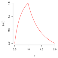
4.10 example: Exponential Distribution
Suppose that
represents the lifetime (thousands of hours) of an incandescent light bulb, such that,
for ,
, for some given
number : note that, as
decreases toward 0, and
increases without limit,
approaches 1. Focus on
a particular number ,
and consider the ratio
for some . As
decreases to
this ratio approaches
. Therefore,
the function
such that is the
probability density of the exponential distribution. In this case, the probability distribution
function is
such that .
’s mean value
is , and its
variance is .
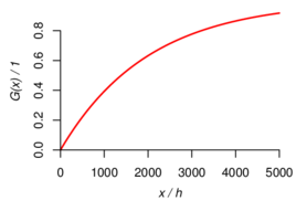
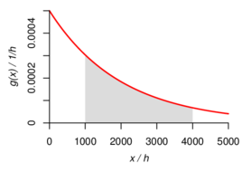
Figure 1 illustrates both the distribution function and the density for the case where
.
Figure 1: Exponential Distribution with Mean 2000 h. The left
panel shows a portion of the graph of the probability distribution
function. The right panel shows the corresponding portion of the graph
of the probability density function. The area of the shaded region
equals the probability of a value between 1000 h and 4000 h: this is
.
Note that the vertical scales in the left and right panels are different.
4.11 Joint, Marginal, and Conditional Distributions
Suppose that
represents a bivariate quantity value, for example, the Cartesian coordinates
of a point inside a circle of unit radius centered at
. In this case
the range
of
is this unit circle. The joint probability distribution of
and
describes a state of knowledge about the location of
: for example, that
more likely than not
is less than ½ away from the center of the circle: statements of this kind involve
and
together (that is, jointly).
The marginal probability distributions of
and
are
the probability distributions that characterize the state of knowledge about each
of them separately from the other: for example, that more likely than not
, irrespective
of .
Clearly, the marginal distributions have to be consistent with the joint
distribution, and while it is true that the joint distribution determines the
marginal distributions, the reverse is not true, in that typically there
are many joint distributions consistent with given marginal distributions
[Possolo, 2010].
Now, suppose one knows that .
This implies that , hence
that is somewhere
on a particular chord
of the unit circle. The conditional probability distribution of
given
that
is a (univariate) probability distribution over this chord.
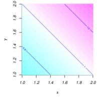
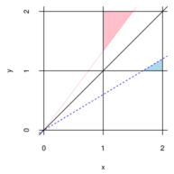
4.12 example: Shark’s Fin
The random variables
and take values in the
interval and have joint
probability density function
such that for
and is zero otherwise
(Figure 2): since
and ,
is a
bona fide (bivariate) probability density.
The density of the marginal distribution of
is
, and
similarly for .
And the density of the conditional distribution of
given
is
.
To determine the probability density of
, also depicted in
Figure 2, note that .
First, consider the case :
and
. Next, consider
the case :
and
.
Figure 2: Shark’s Fin. The left panel shows
the probability density of the joint distribution of
and
defined in §4.12. In the middle panel, the dashed (blue) line has slope
,
and the points inside the small (blue) triangle
have coordinates that satisfy the conditions
and .
The dotted (red) line has slope ,
and the points inside the large (red) triangle
have coordinates that satisfy the conditions
and .
The right panel shows the probability density function of
.
4.13 Independent Random Variables
The (scalar or vectorial) random variables
and
are independent
if and only if
for all
subsets
and
in their respective ranges (to which probabilities can be coherently assigned.)
Suppose
and
have joint probability distribution with probability density function
, and marginal
density functions
and :
the random variables are independent if and only if
.
4.14 example: Unit Circle
Suppose that the probability distribution of a point is
uniform inside the circle of unit radius centered at the origin
of the
Euclidean plane. This means that the probability that a point with Cartesian coordinates
should lie in a subset
of this circle is proportional
to ’s area, but is otherwise
independent of ’s
shape or location within the circle. The probability density function of the joint distribution
of and
is the
function
such that
if , and
otherwise. The
random variables
and
are dependent (§4.13): for example, if one is told that
, then one can surely
conclude that . The
marginal distribution of
has density
such that
for .
has expected value 0 and standard deviation ½. Owing to symmetry,
and
have
identical marginal distributions.
4.15 Correlations and Copulas
If two or more of the random variables are dependent, then modeling their
individual probability distributions will not suffice to specify their joint behavior:
their joint probability distribution is needed.
One commonly used metric of dependence between two random variables
and
is Pearson’s product-moment correlation coefficient, defined as
.
However, it is possible for the variables to be dependent and still have
.
When the only information in hand are the expected values, standard deviations,
and correlations, and still one needs a joint distribution consistent with this
information, then the usual course of action is to assign distributions to them
individually, and then manufacturing a joint distribution using a copula
[Possolo, 2010] — there is, however, a multitude of different copulas that can be
used for this purpose, and the choice that must be made generally is
influential.
5 Functions of Random Variables
5.1 Overview
If a random variable
is a function of other random variables,
, then
and the joint probability
distribution of determine the
probability distribution of .
If only the means, standard deviations, and correlations of
are known,
then it still is possible to derive approximations to the mean and standard deviation
of , by
application of the Delta Method.
If the joint probability distribution of
is
known, then it may be possible to determine the probability distribution of
analytically, using the change of variables formula.
In general, it is possible to obtain a sample from
’s
distribution by taking a sample from the joint distribution of
and
applying
to each element of this sample (§5.8). The results may then be summarized in
several different ways: one of them is an estimate of the probability density of
[Silverman, 1986], a procedure that is implemented in function density of the R
environment for statistical programming and graphics [R Development Core
Team, 2010].
5.2 Delta Method
If is a random
variable with mean
and variance ,
is a
differentiable real-valued function of a real variable whose first derivative does not
vanish at ,
and ,
then ,
and .
(This results from the so-called Taylor approximation that replaces
by a straight line
tangent to its graph at .)
If is an
average of independent, identically distributed random variables with finite variance, then
also is approximately
Gaussian with mean
and standard deviation ,
where
denotes the absolute value of the first derivative of
evaluated
at .
The quality of the approximation improves with increasing
.
5.3 Delta Method — Degeneracy
When and
exists and
is not zero,
is an average of independent, identically distributed random variables with finite variance,
and
is large, then the probability distribution of
is approximately
like that of , where
denotes a Gaussian
(or, normal) random variable with mean 0 and standard deviation 1. Since the variance of
is 2, the standard
deviation of is
approximately ,
rather different from what applies in the conditions of §5.2.
5.4 example: Radiant Power
Consider a surface whose reflectance is Lambertian: that is, light falling on it is
scattered in such a way that the surface’s brightness apparent to an observer is
the same regardless of the observer’s angle of view. The radiant power
emitted by such surface that is measured by a sensor aimed at angle
to the surface’s normal
is proportional to ,
hence one writes
[Cannon, 1998, Köhler, 1998].
If knowledge about the value of
is modeled by a Gaussian distribution with mean
and standard
measurement uncertainty
(both expressed in radians), then §5.2 (with
) suggests that
knowledge of
should be described approximately by a Gaussian distribution with mean
and standard
measurement uncertainty .
If, for example, ,
, and
, then the
approximation to ’s
distribution that the Delta Method suggests, of a Gaussian distribution with mean
and standard
deviation ,
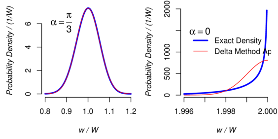
is remarkably accurate (Figure 3).
When the detector is aimed squarely at the target, that is
, this
approximation no longer works because the first derivative of the cosine vanishes
at ,
which is the degenerate case that §5.3 contemplates. In this case,
’s
standard measurement uncertainty is approximately
. For
and
, this
equals ,
which is accurate to the two significant digits shown. However, Figure 3 shows
that, in this case, the Delta Method produces a poor approximation.
When , the
probability density of
is markedly asymmetrical, and the meaning of
’s
standard deviation is rather different from its meaning when
. Indeed,
when the
probability that
should lie within one standard deviation of its expected value is
approximately.
Figure 3: Radiant Power. Probability density of the radiant power
emitted by a Lambertian surface that is
measured by a sensor aimed at an angle
to the surface’s normal, when
has a Gaussian distribution with mean
(left panel) or
(right panel), and standard deviation .
In both cases, the thick blue line is the exact density, and the thin red line
is the Delta Method approximation.
5.5 Delta Method — Multivariate
The Delta Method can be extended to apply to a function of several random variables.
Suppose that ,
…,
are averages of sets of random variables whose variances are finite. The
variables in each set are independent and identically distributed, those in set
having
mean and
variance .
However, variables in different sets may be dependent, hence the
may be dependent,
too. Let denote the
symmetrical matrix
whose element
is the covariance
between
and ,
for .
Now, consider the random variable ,
where denotes a
real-valued function of
variables whose first partial derivatives are continuous and none vanishes at
. If
is finite, then
also is approximately
Gaussian with mean
and variance .
If are uncorrelated
and have means and
standard deviations ,
then the Delta Method approximation reduces to a well-known
formula first presented by Gauss [Gauss, 1823, §18, Problema]:
, where the sensitivitycoefficient is
the value at of
the th partial
derivative of
with respect to .
5.6 example: Beer-Lambert-Bouguer Law
If a beam of monochromatic light of power
(W) travels a
path of length
(m) through a solution containing a solute whose molar absorptivity for that light
is
(L mol-1 m-1), and whose molar concentration is
(mol L-1), then the beam’s power is reduced to
(W) such that
. Application of Gauss’s
formula (§5.5) to
yields:
5.7 example: Darcy’s Law
Darcy’s law relates the dynamic viscosity
of a fluid to the volumetric
rate of discharge
(volume per unit of time) when the fluid flows through a permeable cylindrical medium of cross-section
and intrinsic
permeability under
a pressure drop of
along a length ,
as follows: .
To compute an approximation to the standard deviation of
, one may use
the formula from §5.5 directly, or first take the logarithm of both sides, which linearizes the
relationship, .
Applied to these logarithms, the formula from §5.5 is exact. The approximation is
then done for each term separately, using the univariate Delta Method.
Since ,
and similarly for the other logarithmic terms,
.
In other words, the square of the coefficient of variation of
is
approximately equal to the sum of the squares of the variation coefficients of the
other variables.
5.8 Monte Carlo Method
The Monte Carlo method offers several important advantages over the Delta
Method described in §5.2 and §5.5: (i) it can produce as many correct
significant digits in its results as may be required; (ii) it does not involve the
computation of derivatives, either analytically or numerically; (iii) it is
applicable in many situations where the Delta Method is not; (iv) it provides a
picture of the whole probability distribution of a function of several random
variables, not just an approximation to it, or to its mean and standard
deviation.
The Monte Carlo method in general dates back to the middle of the twentieth
century [Metropolis and Ulam, 1949, Metropolis et al., 1953]. A variant used in
mathematical statistics is known as the parametric bootstrap [Efron and
Tibshirani, 1993]. This involves using random draws from a (possibly
multivariate) probability distribution whose parameters have been replaced by
estimates thereof (for example, means of posterior probability distributions, §6) to
ascertain the probability distribution of a function of one (or more) random
variables. Morgan and Henrion [1992] and Joint Committee for Guides in
Metrology [2008b] describe how it may be employed to evaluate measurement
uncertainty, and provide illustrative examples.
The procedure comprises the following steps:
MC1
Define the joint probability distribution of ,
…, .
MC2
Choose a suitably large positive integer
and draw a sample of size
from this joint distribution to obtain ,
…, .
(If ,
…,
happen to be independent, then this amounts to drawing a sample of
size
from the distribution of each of them separately.)
MC3
Compute ,
…, ,
which are a sample from ’s
distribution.
MC4
Summarize this sample in one or more of these different ways:
MC4.a — Probability Density
The most inclusive summarization
is in the form of an estimate of ’s
probability density function: this may be either a simple histogram,
or a kernel density estimate [Silverman, 1986].
MC4.b — Mean and Standard Deviation
The mean and standard
deviation of
are estimated by the mean and the standard deviation of .
(To ascertain the number of significant digits in this mean and
standard deviation, hence to decide whether
is large enough for the intended purpose, or should be increased,
one may employ either the adaptive procedure explained in the
Supplement 1 to the GUM [Joint Committee for Guides in Metrology, 2008b,
7.9], or resort to the non-parametric statistical bootstrap or to
other resampling methods [Davison and Hinkley, 1997].)
MC4.c — Probability Interval
If
denote the result of ordering
from smallest to largest, then the interval
includes ’s
true value with probability .
(Since
and
need not be integers, the end-points of this coverage interval may
be calculated by interpolation of adjacent s.)
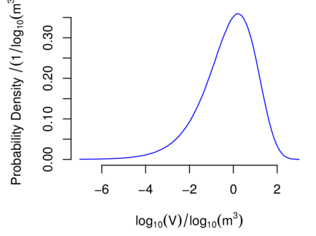
5.9 example: Volume of Cylinder
The radius
and the height
of a cylinder are values of independent random variables with exponential probability
distributions with mean 1 m. To characterize the probability distribution of its volume
, draw a sample of
size from the joint
distribution of
and ,
and compute the volume corresponding to each pair of sampled values
to obtain a sample of the same size from the distribution of
. The
average and standard deviation of these values are 6.3 m3 and 21 m3, and they are
estimates (whose two most significant digits are exact) of the mean and standard
deviation of .
Figure 4 depicts an estimate of the corresponding probability density.
Figure 4: Cylinder Volume. Kernel density estimate [Silverman, 1986] of
the probability density of the volume of a cylinder whose radius and height are
realized values of independent, exponentially distributed random variables
with mean 1 m.
5.10 Change-of-Variable Formula — Univariate
Suppose that
is a random variable with a continuous distribution and values in
, with probability distribution
function and probability
density function , and
consider the random variable
where
denotes a real-valued function of a real variable. Let
denote the set
where takes its
values, and let
and
denote ’s
probability distribution function and probability density function, respectively. In
these circumstances [Casella and Berger, 2002, Chapter 2].
If
is increasing on
and
denotes its inverse, then
for ;
and if
is decreasing, then .
If
is either increasing or decreasing on
(but not both), and its inverse
has a continuous first derivative ,
then ,
for ,
where
denotes the absolute value of the derivative of
at .
5.11 example: Oscillating Mirror
A horizontal beam of light emerges from a tiny hole in a wall and travels along a
1 m long path at right angles to the wall, towards a flat mirror that oscillates
freely around a vertical axis. When the mirror’s surface normal makes an angle
with the beam, its reflection hits the wall at distance
from
the hole (positive to the right of the hole and negative to the left). If
is uniformly (or, rectangularly) distributed between
and
, then
, and
’s probability
density is
such that
for .
As it turns out, both the mean and the standard deviation of
are
infinite [Feller, 1971, Page 51].
5.12 Change-of-Variable Formula — Multivariate
Suppose that are random
variables and consider
for , and where
are real-valued
functions of
real variables each.
Suppose also that (i) the vector
takes values in an open subset
of -dimensional
Euclidean space, and has a continuous joint probability distribution with probability density function
; (ii) the vector-valued
function is invertible,
and the inverse has a
Jacobian determinant
that does not vanish on .
CV1
Solve the
equations ,
…, ,
for ,
to obtain the inverse transformation such that ,
…, .
CV2
Find , the partial
derivative of with
respect to its th
argument, for ,
and compute the Jacobian determinant of the inverse transformation at
:
CV3
The density the joint probability distribution of the random vector
is
such that
(2)
Note that is
a scalar, and
denotes its absolute value.
CV4
The probability density of
is , where the
integrals are over
the ranges of .
5.13 example: Linear Combinations of Gaussian Random Variables
Suppose that
and
are independent, Gaussian random variables with mean 0 and variance 1, and let
, and
, for given real
numbers and
. The inverse
transformation maps
onto , and has Jacobian
determinant whose
absolute value is .
Since the density of the joint probability distribution of
and
is
,
application of the multivariate change-of-variable formula yields
But this means that
and
also are independent and Gaussian with mean 0 and variance
.
On the one hand, this result is surprising because
and
both are functions of the same random variables. On the other hand it is
hardly surprising because the transformation amounts to a rotation of the
coordinate axes, followed by a global dilation. Since the joint distribution of
and
is circularly symmetric
relative to , so will the
joint distribution of
and
be, which implies independence and the same functional form for the density, up
to a difference in scale.
5.14 example: Ratio of Exponential Lifetimes
To compute the probability density of the ratio
of two independent and exponentially distributed random variables
and
with mean
, define the
function such that
, whose inverse is
, with Jacobian
determinant .
The multivariate change-of-variable formula then yields
for the density of the
joint distribution of
and . The (marginal)
density of
is , for
,
being 0 otherwise.
indeed is a probability density function because it is a non-negative function and
. However, since
, neither the mean
nor the variance of
is finite. The Delta Method, however, would have suggested that
and
that the coefficient of variation (ratio of the standard deviation to the mean) of
is
approximately.
5.15 example: Polar Coordinates
The inverse of the transformation that maps the polar coordinates
of a point in the Euclidean plane to its Cartesian coordinates
is
such
that for
and
, with Jacobian
determinant .
If and
are
independent Gaussian random variables with mean 0 and variance 1, then the probability
density of
is . Since
, it follows
that
and
are independent, the former having a Rayleigh distribution with mean
, the latter a uniform
distribution between
and .
6 Statistical Inference
The statistical inferences we are primarily interested in are probabilistic
statements about the unknown value of a quantity, produced by application of a
statistical method. In the example of §6.6, one of the inferences is this statement:
the probability is 95% that the difference between the numbers of hours gained withthe two soporifics is between 0.7 h and 2.5 h.
Another common inference is an estimate of the value of a quantity, which must be
qualified with an assessment of the associated uncertainty. In the example of §6.8, a
typical inference of this kind would be this: the difference in mean levels of thyroxinein the serum of two groups of children diagnosed with hypothyroidism is estimated aswith standarduncertainty
(Figure 6).
In our treatment of this example, the inference is based entirely on a small set of
empirical data, and on a particular choice of statistical model used to describe the
dispersion of the data, and to characterize the fact that no knowledge other than
the data was brought into play.
Statistical methods different from the one we used could have been employed:
some of these would produce the same result (in particular those illustrated when
this dataset was first described [Student, 1908, Fisher, 1973]), while others would
have produced different results.
Even when the result is the same, it may be variously interpreted:
For some that statement means that if the same sampling and study
method is used repeatedly, and each time the resulting dataset is
modeled and analyzed in the same way to produce an interval like the
one above, then about 95 % of the resulting intervals will include the
true difference sought — with no guarantee or implication that the
interval that was obtained is one of these;
For others (among whom we stand) that statement expresses the degree
of belief one is entitled to have about the true difference lying between
0.7 h and 2.5 h specifically, in light of all the relevant information in
hand.
6.1 Bayesian Inference
Bayesian inference [Bernardo and Smith, 2000, Lindley, 2006, Robert, 2007] is a
class of statistical procedures that serve to blend preexisting information about
the value of a quantity with fresh information in empirical data.
The defining traits of a Bayesian procedure are these:
(i)
All quantity values that are the objects of interest but are accessible
to direct observation (non-observables) are modeled as values of
non-observable random variables whose (prior, or a priori) distributions
encode and convey states of incomplete knowledge about those values;
(ii)
The empirical data (observables) are modeled as realized values of
random variables whose probability distributions depend on those
objects of interest;
(iii)
Preexisting information about those objects of interest is updated in
light of the fresh empirical data by application of Bayes rule, and the
results are encapsulated in a (posterior, or a posteriori) probability
distribution;
(iv)
Selected aspects of this distribution are then abstracted from it and
used to characterize the objects of interest and to describe the state of
knowledge about them.
6.2 Prior Distribution
Let denote
the value of the quantity of interest, which we model as realized value of a random variable
with probability density
function that encodes the
state of knowledge about
prior to obtaining fresh data, and which must be defined even if there is no prior
knowledge.
Defining such
often is a challenging task. If in fact there exists substantial prior knowledge about
, then
it needs to be elicited from experts in the matter and encapsulated in the form of
a particular probability density: Garthwaite et al. [2005] review how
this may be done. For example, when measuring the mass fraction of
titanium in a mineral specimen, then knowledge of the species (ilmenite,
titanite, rutile, etc.) of the specimen is highly informative about that mass
fraction. Familiarity with the process of analytical chemistry employed
to make the measurement may indicate the dispersion of values to be
expected.
In some cases, essentially no prior knowledge exists about
, or
none is deemed reliable enough to be taken into account. In such cases, a so-called
non-informative prior distribution needs to be produced and assigned to
that reflects this
state of affairs: if
is univariate (that is, a single number), then the rules developed by Jeffreys [1961] often prove
satisfactory; if
is multivariate (that is, a numerical vector), then the so-called reference prior
distributions are recommended [Bernardo and Smith, 2007] (these reduce to
Jeffreys’s in the univariate case).
These rules often produce a that
is improper, in the sense that
diverges to infinity, where
denotes the range of .
(If
should have a discrete distribution then this integral is replaced by a sum.)
Fortunately, once used in Bayes Rule (§3.5 and §6.4), improper priors often lead
to proper posterior probability distributions.
6.3 Likelihood Function
The empirical data
(which may be a single number, a numerical vector, or a data structure of still
greater complexity) are modeled as realized values of a random variable
whose probability density describes the corresponding dispersion of values.
This density must depend on ,
which is another way of saying that the data are informative about
(otherwise there would be nothing to be gained by observing them). In
fact, this is the density of the conditional probability distribution of
given
that .
Choosing a specific functional form for it generally is a non-trivial exercise: it
involves defining a statistical model that correctly captures the dispersion of
values likely to be obtained in the experiment that produces them.
Once the data are
in hand, becomes a
function of alone, being
largest for values of
that make the data appear most likely. As such, it still is non-negative, but its integral (or
sum, if ’s
distribution should be discrete) over the range of
, need
not be 1.
6.4 Posterior Distribution
Suppose that both
given that and
have continuous
distributions with densities
and .
In these circumstances, Bayes rule becomes
(3)
The function , which is
defined over the range of
for each fixed value ,
is the density of the posterior distribution of the value of the quantity of interest
given
the data.
In some cases this can be computed in closed form, in many others it cannot. In
all cases it is possible to obtain a sample from this posterior distribution by
application of a procedure known as Markov Chain Monte Carlo (MCMC)
[Gelman et al., 2003]. This sample can then be summarized as described in
§5.8.
6.5 example: Viral Load
Once infected by influenza A virus, an epithelial cell of the upper respiratory tract
releases
virions on average, which may then go on to infect other cells. This number
depends
on the volume of the cell, and we will treat it as realized value of a non-observable
random variable with an exponential distribution whose expected value,
for some
, is known.
Given ,
the actual number of virions that are released is
,
and this is like a realized value of a Poisson random variable with mean
.
Suppose that the prior density is ,
and the likelihood function is ,
for . The posterior
distribution of
given
belongs to the gamma family, and has expected value
, variance
, and
density
6.6 example: Sleep Hours
The differences between the numbers of additional hours of sleep that ten patients
gained when using two soporific drugs, described in examples given by
Student [1908] and [Fisher, 1973, §24], were 1.2 h, 2.4 h, 1.3 h, 1.3 h, 0.0 h, 1.0 h,
1.8 h, 0.8 h, 4.6 h, and 1.4 h.
Suppose that, given
and ,
these are realized values of independent Gaussian random variables with mean
and variance
. Let
denote their
average, and
denote the sum of their squared deviations from
divided by 9. In these circumstances, the likelihood function is
.
Assume, in addition, that
and
are realized values of non-observable random variables
and
that are independent
a priori and such that
and are uniformly
distributed between
and
(both improper prior distributions). Then, given
and
,
is like a realized value of a random variable with a Student’s
distribution
with degrees
of freedom, and
is like a realized value of a random variable with a chi-squared distribution with
degrees of freedom [Box and Tiao, 1973, Theorem 2.2.1].
Therefore, the expected value of the posterior distribution
of the mean difference of hours of sleep gained is
, and the standard
deviation is . A 95 %
probability interval for
ranges from 0.7 h to 2.5 h, and a similar one for
ranges from 0.8 h to 2.2 h.
Suppose that
and are the
counterparts of
and
once the information in the data has been taken into account:
that is, their probability distribution is the joint (or, bivariate)
posterior probability distribution given the data. Even though
and
were assumed to be
independent a priori,
and
turn out to be dependent a posteriori (that is, given the data), but their
correlation is zero [Lindley, 1965b, §5.4].
6.7 example: Hurricanes
A major hurricane has category 3, 4, or 5 on the Saffir-Simpson Hurricane Scale
[Simpson, 1974]: its central pressure is no more than 945 mbar (94 500 Pa), it has winds
of at least
(49.6 m s-1), generates sea surges of 9 feet (2.7 m) or greater, and has the
potential to cause extensive damage.
The numbers of major hurricanes that struck the U.S. mainland directly, in
each decade starting with 1851–1860 and ending with 1991–2010, are:
6, 1, 7, 5, 8, 4, 7, 5, 8, 10, 8, 6, 4, 4, 5, 7 [Blake et al., 2011]. Let
denote the number of decades,
denote the corresponding
counts, and . Suppose that
one wishes to predict ,
the number of such hurricanes in the decade 2011–2020.
Assume that the mean number of such hurricanes per decade will have remained constant
between 1851 and 2010 (certainly a questionable assumption), with unknown value
, and that, conditionally
on this value, ,
…, ,
and
are realized values of independent Poisson random variables
, …,
(observable),
(non-observable), all with
mean value : their common
probability density is
for .
This model is commonly used for phenomena that result from the cumulative
effect of many improbable events [Feller, 1968, XI.6b].
Even though the goal is to predict ,
the fact that there is no a priori knowledge about
other than
that it must be positive, requires that this be modeled as the (non-observable) value of a
random variable
whose probability distribution must reflect this ignorance. (According to the
Bayesian paradigm, all states of knowledge, even complete ignorance, have to be
modeled using probability distributions.)
If the prior distribution chosen for
is the reference prior distribution [Berger, 2006, Bernardo, 1979, Bernardo
and Smith, 2000], then the value of its probability density
at
should be
proportional to
[Bernardo and Smith, 2000, A.2], an improper prior probability
density. However, the corresponding posterior distribution for
is proper, in fact it is a gamma distribution with expected value
and probability
density function
such that
(4)
However, what is needed for the aforementioned prediction is the conditional distribution
of given
the observed counts: the so-called predictive distribution [Schervish, 1995, Page 18].
If
denotes the corresponding density, then
This defines a discrete probability distribution on the non-negative integers, often called
a Poisson-gamma mixture distribution [Bernardo and Smith, 2000, §3.2.2]. For our data,
since achieves
a maximum at
(Figure 5), this is the (a posteriori) most likely number
of major hurricanes
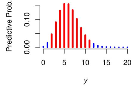
that will hit the U.S. mainland in 2011–2020. The mean of the posterior distribution is
. Since the probability
is 0.956 that ’s
value lies between 2 and 11 (inclusive), the interval whose end-points are 2 and 11 is a
coverage
interval for .
Figure 5: Hurricanes. Predictive probabilities for the number of major
hurricanes that
will hit the U.S. mainland in 2011–2020. The vertical axis indicates values of
from equation (5). The most likely number is 5, the expected number is
6, and the probability is 0.956 that the number will be between 2 and 11
(inclusive) (red bars).
6.8 example: Hypothyroidism
[Altman, 1991, Table 9.6] lists measurement results from Hulse et al. [1979], for
the concentration of thyroxine in the serum of sixteen children diagnosed
with hypothyroidism, of which nine had slight or no symptoms, and the
other seven had marked symptoms. The values measured for the former,
all in units of nmol/L, were 34, 45, 49, 55, 58, 59, 60, 62, and 86; and
for the latter they were 5, 8, 18, 24, 60, 84, and 96. The averages are
and
, and the standard
deviations are
and .
Our goal is to produce a probability interval for the difference between the corresponding
means,
and ,
say, when nothing is assumed known a priori either about
these means or about the corresponding standard deviations,
and
,
which may be different.
Given the values of these four parameters, suppose that the values measured in the
children with
slight or no symptoms are observed values of independent Gaussian random variables
with common
mean and standard
deviation , and that
those measured in the
children with marked symptoms are observed values of independent Gaussian random variables
, also independent
of the , with
common mean and
standard deviation .
The problem of constructing a probability interval for
under these circumstances is known as the Behrens-Fisher problem
[Ghosh and Kim, 2001]. For the Bayesian solution, we regard
,
,
and
as realized values of non-observable random variables
,
,
, and
, assumed independent
a priori and such that ,
,
, and
all
are uniformly distributed over the real numbers (hence have improper prior
distributions). The corresponding posterior distributions all are proper provided
and
.
However, the density of the posterior probability distribution of
given
the data cannot be computed in closed form.
This problem in Bayesian inference, and other problems much more demanding
than this, can be solved using the MCMC sampling technique mentioned in
§6.4, for which there exist several generic software implementations: we
obtained the results presented below using function metrop of the R package
mcmc [Geyer, 2010]. Typically, all that is needed is the logarithm of the
numerator of Bayes formula (3). Leaving out constants that do not involve
,
,
or
, this
is
MCMC produces a sample of suitably large size
from the joint posterior
distribution of ,
,
, and
, given the
data, say ,
…, .
The 95 % probability interval for the difference in mean levels of
thyroxine in the serum of the two groups, which extends from
to
, and Figure 6, are based
on a sample of size .
The probability density in this figure, and that probability interval, were computed
as described in MC4.c and MC4.d of §5.8, only applied to the differences
.
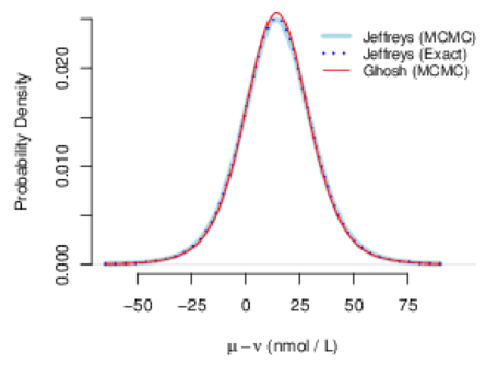
Figure 6: Hypothyroidism. Probability density of the posterior
distribution of the difference in mean levels of thyroxine in the serum
of two groups of children diagnosed with hypothyroidism: computed
via MCMC using either Jeffreys’s prior or the “matching” prior of
Ghosh and Kim [2001], alongside the exact version corresponding
to Jeffreys’s prior. The posterior mean and standard deviation are
and .
In this particular case it is possible to ascertain the correctness of the results owing to an
interesting, albeit surprising result: the posterior means are independent a posteriori,
and have probability distributions that are re-scaled, shifted versions of Student’s
distributions
with
and
degrees of freedom [Box and Tiao, 1973, 2.5.2]. Therefore, by application of the Monte
Carlo method of §5.8, one may obtain a sample from the posterior distribution of the
difference
independently of the MCMC procedure: the results are depicted in Figure 6
(where they are labeled “Jeffreys (Exact)”), and are essentially indistinguishable
from the results of MCMC.
This same figure shows yet another posterior density that differs hardly
at all from the posterior density corresponding to Jeffreys’s prior: this
alternative result corresponds to the “matching” prior distribution (also
improper) derived by Ghosh and Kim [2001], whose density is proportional to
. This
illustrates a generally good practice: that the sensitivity of the results of Bayesian
analysis should be evaluated by comparing how they vary when different but
comparably acceptable priors are used.
7 Acknowledgments
Antonio Possolo thanks colleagues and former colleagues from the Working Group
1 of the Joint Committee for Guides in Metrology, who offered valuable
comments and suggestions in multiple discussions of an early draft of a
document that he had submitted to the consideration of this Working
Group and that included material now in the present document: Walter
Bich, Maurice Cox, René Dybkær, Charles Ehrlich, Clemens Elster,
Tyler Estler, Brynn Hibbert, Hidetaka Imai, Willem Kool, Lars Nielsen,
Leslie Pendrill, Lorenzo Peretto, Steve Sidney, Adriaan van der Veen,
Graham White, and Wolfgang Wöger. Antonio Possolo is particularly
grateful to Tyler Estler for suggestions regarding §2.3 and §3.1, and to
Graham White for suggestions and corrections that greatly improved §3.6, on
the tuberculin test. Both authors thank their common NIST colleagues
Andrew Rukhin and Jack Wang for suggesting many corrections and
improvements. Mary Dal-Favero and Alan Heckert, both from NIST,
kindly facilitated the deployment of this material on the World Wide
Web.
References
D. G. Altman. Practical Statistics for Medical Research. Chapman &
Hall/CRC, Boca Raton, FL, 1991. Reprinted 1997.
American Thoracic Society. Diagnostic standards and classification of
tuberculosis in adults and children. American Journal of Respiratory andCritical Care Medicine, 161:1376–1395, 1999.
J. Berger. The case for objective Bayesian analysis. Bayesian Analysis,
1(3):385–402, 2006. URL http://ba.stat.cmu.edu/.
J. Bernardo and A. Smith. Bayesian Theory. John Wiley & Sons, New
York, 2000.
J. Bernardo and A. Smith. Bayesian Theory. John Wiley & Sons,
Chichester, England, 2nd edition, 2007.
J. M. Bernardo. Reference posterior distributions for Bayesian inference.
Journal of the Royal Statistical Society, 41:113–128, 1979.
E. S. Blake, C. W. Landsea, and E. J. Gibney. The deadliest, costliest,
and most intense United States tropical cyclones from 1851 to 2010 (and
other frequently requested hurricane facts). Technical Report Technical
Memorandum NWS NHC-6, NOAA, National Weather Service, National
Hurricane Center, Miami, Florida, August 2011.
L. Bovens and W. Rabinowicz. Democratic answers to complex
questions — an epistemic perspective. Synthese, 150:131–153, 2006.
G. E. P. Box and G. C. Tiao. Bayesian Inference in Statistical Analysis.
Addison-Wesley, Reading, Massachusetts, 1973.
T. W. Cannon. Light and radiation. In C. DeCusatis, editor, Handbookof Applied Photometry, chapter 1, pages 1–32. Springer Verlag, New York,
New York, 1998.
R. Carnap. Logical Foundations of Probability. University of Chicago
Press, Chicago, Illinois, 2nd edition, 1962.
G. Casella and R. L. Berger. Statistical Inference. Duxbury, Pacific
Grove, California, 2nd edition, 2002.
N. Clee. Who’s the daddy of them all? In Observer Sport Monthly.
Guardian News and Media Limited, Manchester, UK, Sunday March 4,
2007.
R. T. Clemen and R. L. Winkler. Combining probability distributions
from experts in risk analysis. Risk Analysis, 19:187–203, 1999.
R. T. Cox. Probability, frequency and reasonable expectation. AmericanJournal of Physics, 14:1–13, 1946.
R. T. Cox. The Algebra of Probable Inference. The Johns Hopkins Press,
Baltimore, Maryland, 1961.
A. C. Davison and D. Hinkley. Bootstrap Methods and theirApplications. Cambridge University Press, New York, NY, 1997.
B. de Finetti. La prévision: ses lois logiques, ses sources subjectives.
Anales de l’Institut Henri Poincaré, 7:1–68, 1937.
B. de Finetti. Theory of Probability: A critical introductory treatment.
John Wiley & Sons, Chichester, 1990. Two volumes, translated from the
Italian and with a preface by Antonio Machì and Adrian Smith, with a
foreword by D. V. Lindley, Reprint of the 1975 translation.
M. H. DeGroot. A conversation with Persi Diaconis. Statistical Science,
1(3):319–334, August 1986.
M. H. DeGroot and M. J. Schervish. Probability and Statistics.
Addison-Wesley, 4th edition, 2011.
P. Diaconis and D. Ylvisaker. Quantifying prior opinion. In
J. M. Bernardo, M. H. DeGroot, D. V. Lindley, and A. Smith,
editors, Bayesian Statistics, volume 2, pages 163–175. North-Holland,
Amsterdam, 1985.
F. W. Dyson, A. S. Eddington, and C. Davidson. A determination of
the deflection of light by the sun’s gravitational field, from observations
made at the total eclipse of May 29, 1919. Philosophical Transactions of theRoyal Society of London, Series A, Containing Papers of a Mathematicalor Physical Character, 220:291–333, 1920.
B. Efron and R. J. Tibshirani. An Introduction to the Bootstrap.
Chapman & Hall, London, UK, 1993.
W. Feller. An Introduction to Probability Theory and Its Applications,
volume I. John Wiley & Sons, New York, 3rd edition, 1968. Revised
Printing.
W. Feller. An Introduction to Probability Theory and Its Applications,
volume II. John Wiley & Sons, New York, 2nd edition, 1971.
R. A. Fisher. Statistical Methods for Research Workers. Hafner
Publishing Company, New York, NY, 14th edition, 1973.
B. Fitelson. Likelihoodism, bayesianism, and relational confirmation.
Synthese, 156(3):473–489, 2007.
P. H. Garthwaite, J. B. Kadane, and A. O’Hagan. Statistical methods
for eliciting probability distributions. Journal of the American StatisticalAssociation, 100:680–701, June 2005.
C. F. Gauss. Theoria combinationis observationum erroribus minimis
obnoxiae. In Werke, Band IV . Könighlichen Gesellschaft der
Wissenschaften, Göttingen, 1823.
A. Gelman, J. B. Carlin, H. S. Stern, and D. B. Rubin. Bayesian DataAnalysis. Chapman & Hall / CRC, 2nd edition, 2003.
M. Ghosh and Y.-H. Kim. The Behrens-Fisher problem revisited: A
Bayes-Frequentist synthesis. The Canadian Journal of Statistics, 29(1):
5–17, March 2001.
D. Gillies. Philosophical Theories of Probability. Routledge, London,
UK, 2000.
C. Glymour. Theory and evidence. Princeton University Press,
Princeton, New Jersey, 1980.
A. Hájek. Interpretations of probability. In E. N.
Zalta, editor, The Stanford Encyclopedia of Philosophy. The
Metaphysics Research Lab, Center for the Study of Language and
Information, Stanford University, Stanford, California, 2007. URL
http://plato.stanford.edu/archives/win2007/entries/probability-interpret/.
P.G. Hoel, S. C. Port, and C. J. Stone. Introduction to ProbabilityTheory. Houghton Mifflin, 1971a.
P.G. Hoel, S. C. Port, and C. J. Stone. Introduction to StatisticalTheory. Houghton Mifflin, 1971b.
M. Holden, M. R. Dubin, and P. H. Diamond. Frequency of negative
intermediate-strength tuberculin sensitivity in patients with active
tuberculosis. New England Journal of Medicine, 285:1506–1509, 1971.
J. A. Hulse, D. Jackson, D. B. Grant, P. G. H. Byfield, and
R. Hoffenberg. Different measurements of thyroid function in hypothyroid
infants diagnosed by screening. Acta Pædiatrica, 68:21–25, 1979.
E. T. Jaynes. Probability Theory in Science and Engineering.
Colloquium Lectures in Pure and Applied Science, No. 4. Socony Mobil
Oil Company, Dallas, Texas, 1958.
E. T. Jaynes. Probability Theory: The Logic of Science. Cambridge
University Press, Cambridge, UK, 2003. G. L. Bretthorst, Editor.
H. Jeffreys. Theory of Probability. Oxford University Press, London, 3rd
edition, 1961. Corrected Impression, 1967.
Joint Committee for Guides in Metrology. Evaluation of measurementdata — Guideto the expression of uncertainty in measurement. International Bureau of
Weights and Measures (BIPM), Sèvres, France, September 2008a. URL
http://www.bipm.org/en/publications/guides/gum.html. BIPM,
IEC, IFCC, ILAC, ISO, IUPAC, IUPAP and OIML, JCGM 100:2008,
GUM 1995 with minor corrections.
Joint Committee for Guides in Metrology. Evaluation of measurementdata — Supplement 1 to the “Guide to the expression of uncertainty inmeasurement” —Propagation of distributions using a Monte Carlo method. International
Bureau of Weights and Measures (BIPM), Sèvres, France, 2008b. URL
http://www.bipm.org/en/publications/guides/gum.html. BIPM,
IEC, IFCC, ILAC, ISO, IUPAC, IUPAP and OIML, JCGM 101:2008.
Joint
Committee for Guides in Metrology. International vocabulary of metrology— Basic and general concepts and associated terms (VIM). International
Bureau of Weights and Measures (BIPM), Sèvres, France, 2008c. URL
http://www.bipm.org/en/publications/guides/vim.html. BIPM,
IEC, IFCC, ILAC, ISO, IUPAC, IUPAP and OIML, JCGM 200:2008.
R. Köhler. Photometric and radiometric quantities. In C. DeCusatis,
editor, Handbook of Applied Photometry, chapter 2, pages 33–54. Springer
Verlag, New York, New York, 1998.
D. Lindley. Understanding Uncertainty. John Wiley & Sons, Hoboken,
New Jersey, 2006.
D. V. Lindley. Introduction to Probability and Statistics from a BayesianViewpoint — Part 1, Probability. Cambridge University Press, Cambridge,
UK, 1965a.
D. V. Lindley. Introduction to Probability and Statistics from a BayesianViewpoint — Part 2, Inference. Cambridge University Press, Cambridge,
UK, 1965b.
D. V. Lindley. Reconciliation of probability distributions. OperationsResearch, 31(5):866–880, September-October 1983.
D. V. Lindley. Making Decisions. John Wiley & Sons, London, 2nd
edition, 1985.
D. H. Mellor. Probability: A Philosophical Introduction. Routledge, New
York, 2005.
N. Metropolis and S. Ulam. The Monte Carlo Method. Journal of theAmerican Statistical Association, 44:335–341, September 1949.
N. Metropolis, A. Rosenbluth, M. Rosenbluth, A. Teller, and E. Teller.
Equations of state calculations by fast computing machines. Journal ofChemical Physics, 21:1087–1091, 1953.
M. G. Morgan and M. Henrion. Uncertainty — A Guide to Dealingwith Uncertainty in Quantitative Risk and Policy Analysis. Cambridge
University Press, New York, NY, first paperback edition, 1992. 10th
printing, 2007.
P. A. Morris. Combining expert judgments: A bayesian approach.
Management Science, 23(7):679–693, March 1977.
J. Neyman. Frequentist probability and frequentist statistics. Synthese,
36(1):97–131, 1977.
K. R. Popper. The propensity interpretation of probability. BritishJournal of the Philosophy of Science, 10:25–42, 1959.
A. Possolo. Copulas for uncertainty analysis. Metrologia, 47:262–271,
2010.
R Development Core Team. R: A Language and Environment forStatistical Computing. R Foundation for Statistical Computing, Vienna,
Austria, 2010. URL http://www.R-project.org. ISBN 3-900051-07-0.
F. P. Ramsey. Truth and probability. In R.B. Braithwaite, editor, TheFoundations of Mathematics and other Logical Essays, chapter VII, pages
156–198. Harcourt,
Brace and Company, New York, 1999 electronic edition, 1926, 1931. URL
http://homepage.newschool.edu/het/texts/ramsey/ramsess.pdf.
H. Reichenbach. The Theory of Probability: An Inquiry into the Logicaland Mathematical Foundations of the Calculus of Probability. University
of California Press, Berkeley, California, 1949. English translation of the
1935 German edition.
C. P. Robert. The Bayesian Choice: From Decision-TheoreticFoundations to Computational Implementation. Springer, New York, NY,
second edition, 2007.
L. J. Savage. The Foundations of Statistics. Dover Publications, New
York, New York, 1972.
M. J. Schervish. Theory of Statistics. Springer Series in Statistics.
Springer Verlag, New York, NY, 1995.
B. W. Silverman. Density Estimation. Chapman and Hall, London, 1986.
R. H. Simpson. The hurricane disaster potential scale. Weatherwise, 27:
169–186, 1974.
M. Stone. The opinion pool. The Annals of Mathematical Statistics, 32:
1339–1342, December 1961.
Student. The probable error of a mean. Biometrika, 6(1):1–25, March
1908.
B. N. Taylor and C. E. Kuyatt. Guidelines for Evaluating andExpressing the Uncertainty of NIST Measurement Results. National
Institute of Standards and Technology, Gaithersburg, MD, 1994. URL
http://physics.nist.gov/Pubs/guidelines/TN1297/tn1297s.pdf.
NIST Technical Note 1297.
R. von Mises. Probability, Statistics and Truth. Dover Publications, New
York, 2nd revised edition, 1981. ISBN 0486242145. Translation of the 3rd
German edition.