HOMOSCEDASTICITY PLOT

HOMOSCEDASTICITY PLOT

Graphics Command

Generates a homoscedasticity plot.

A homoscedasticity plot is a graphical data analysis technique for assessing the assumption of constant variance across subsets of the data. The first variable is a response variable and the second variable identifies subsets of the data. The mean and standard deviation are calculated for each of these subsets. The following plot is generated:

Vertical axis	=	subset standard deviations;
Horizontal axis	=	subset means.

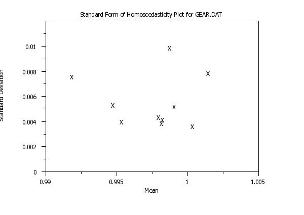
The interpretation of this plot is that the greater the spread on the vertical axis, the less valid is the assumption of constant variance.

By default, this command assumes that you have raw data. In some cases, you may only have summary data (i.e., means and standard deviations or some other location/scale statistics). See Syntax 4 and Syntax 5 for how to use this command with summary data.

You can also use this command when you have more than one group-id variable.

HOMOSCEDASTICITY PLOT <y> <x1> ... <xk>
                        <SUBSET/EXCEPT/FOR qualification>
where <y> is a response variable;
            <x1> ... <xk> is a list of one to six group-id variables;
and where the <SUBSET/EXCEPT/FOR qualification> is optional.

From one to six group-id variables can be specified (most commonly there is a single group-id variable).

Note that with this syntax, all plot points are drawn with the same characteristics (i.e., the first setting of the CHARACTER and LINE commands and their associated attribute setting commands).

SUBSET HOMOSCEDASTICITY PLOT <y> <x1> ... <xk>
                        <SUBSET/EXCEPT/FOR qualification>
where <y> is a response variable;
            <x1> ... <xk> is a list of one to six group-id variables;
and where the <SUBSET/EXCEPT/FOR qualification> is optional.

From one to six group-id variables can be specified (most commonly there is a single group-id variable).

Note that with this syntax, the plot points corresponding to each subset are drawn with different attributes (i.e., the first subset uses the first setting for the CHARACTER and LINE and related attribute setting commands, the second subset uses the second setting, and so on). For example, this syntax can be used to label the plot points with the lab-id.

If there is more than one group-id variable, the attribute settings work from right to left. That is, if X1 has 2 levels and X2 has 2 levels, then

trace 1	=	Level 1 of X1 and Level 1 of X2
trace 2	=	Level 1 of X1 and Level 2 of X2
trace 3	=	Level 2 of X1 and Level 1 of X2
trace 4	=	Level 2 of X1 and Level 1 of X2

MULTIPLE HOMOSCEDASTICITY PLOT <y1> ... <yk>
                        <SUBSET/EXCEPT/FOR qualification>
where <y1> ... <yk> is a list of one to 30 response variables;
and where the <SUBSET/EXCEPT/FOR qualification> is optional.

With this syntax, the different subsets are represented with different response variables. As with Syntax 2, each subset is drawn with different attributes.

SUMMARY HOMOSCEDASTICITY PLOT <ymean> <ysd> <nrepl>
                        <SUBSET/EXCEPT/FOR qualification>
where <ymean> is a variable containing subset means;
            <ysd> is a variable containing subset standard deviations;
            <nrepl> is an optional variable containing the number of replications in each subset;
and where the <SUBSET/EXCEPT/FOR qualification> is optional.

This syntax is used when you only have summary data. The <ymean> variable contains the means (or some other location statistic) and <ysd> contains the standard deviations (or some other scale statistic) for the different subsets.

The <nrepl> variable is only used when the CIRCLE TECHNIQUE is used to generate lines of "similar homogeneity". See the Note section below for a description of the CIRCLE TECHNQUE.

As with Syntax 1, all plot points are drawn with the same attributes.

SUMMARY SUBSET HOMOSCEDASTICITY PLOT <ymean> <ysd> <nrepl>
                        <SUBSET/EXCEPT/FOR qualification>
where <ymean> is a variable containing subset means;
            <ysd> is a variable containing subset standard deviations;
            <nrepl> is an optional variable containing the number of replications in each subset;
and where the <SUBSET/EXCEPT/FOR qualification> is optional.

This syntax is used when you only have summary data. The <ymean> variable contains the means (or some other location statistic) and <ysd> contains the standard deviations (or some other scale statistic) for the different subsets.

The <nrepl> variable is only used when the CIRCLE TECHNIQUE is used to generate lines of "similar homogeneity". See the Note section below for a description of the CIRCLE TECHNQUE.

As with Syntax 2, the different subsets are plotted with different attributes.

HOMOSCEDASTICITY PLOT Y1 TAG
HOMOSCEDASTICITY PLOT Y1 TAG SUBSET TAG > 2
MULTIPLE HOMOSCEDASTICITY PLOT Y1 Y2 Y3 Y4 Y5
MULTIPLE HOMOSCEDASTICITY PLOT Y1 TO Y5
SUBSET HOMOSCEDASTICITY PLOT Y1 TAG
SUMMARY SUBSET HOMOSCEDASTICITY PLOT YMEAN YSD
SUBSET HOMOSCEDASTICITY PLOT Y1 X1 X2

The CHARACTER and LINE commands and their associated attribute setting commands can be used to control the appearance of the plot. See the program examples below for a demonstration of setting the character and line attributes for the various syntaxes described above.

Although the default form of this command plots the standard deviation versus the mean, a number of alternate location and scale statistics can be used.

You can set the location statistic with the commands

SET HOMOSCEDASTICITY LOCATION MEAN
SET HOMOSCEDASTICITY LOCATION BIWEIGHT LOCATION
SET HOMOSCEDASTICITY LOCATION H10
SET HOMOSCEDASTICITY LOCATION H12
SET HOMOSCEDASTICITY LOCATION H15
SET HOMOSCEDASTICITY LOCATION H17
SET HOMOSCEDASTICITY LOCATION H20
SET HOMOSCEDASTICITY LOCATION HODGES LEHMAN
SET HOMOSCEDASTICITY LOCATION LP LOCATION
SET HOMOSCEDASTICITY LOCATION MEDIAN
SET HOMOSCEDASTICITY LOCATION MIDMEAN
SET HOMOSCEDASTICITY LOCATION MIDRANGE
SET HOMOSCEDASTICITY LOCATION TRIMMED MEAN
SET HOMOSCEDASTICITY LOCATION WINSORIZED MEAN


You can set the scale statistic with the commands

SET HOMOSCEDASTICITY SCALE SD (or STANDARD DEVIATION)
SET HOMOSCEDASTICITY SCALE BIWEIGHT SCALE
SET HOMOSCEDASTICITY SCALE H10
SET HOMOSCEDASTICITY SCALE H12
SET HOMOSCEDASTICITY SCALE H15
SET HOMOSCEDASTICITY SCALE H17
SET HOMOSCEDASTICITY SCALE H20
SET HOMOSCEDASTICITY SCALE AVERAGE ABSOLUTE DEVIATION
            (or AAD)
SET HOMOSCEDASTICITY SCALE MEDIAN ABSOLUTE DEVIATION
            (or MAD)
SET HOMOSCEDASTICITY SCALE INTERQUARTILE RANGE (or IQ)
SET HOMOSCEDASTICITY SCALE RANGE
SET HOMOSCEDASTICITY SCALE TRIMMED SD
SET HOMOSCEDASTICITY SCALE WINSORIZED SD
SET HOMOSCEDASTICITY SCALE SN
SET HOMOSCEDASTICITY SCALE QN

The ISO 13528 Standard describes a method for generating confidence contours for homogeneity. That is, for a given level of \( \alpha \), labs outside the confidence contour are not homogeneous with the other labs.

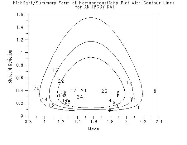
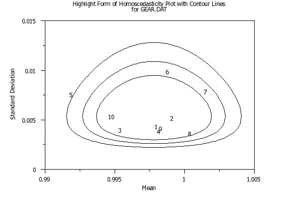
The method used is referred to as the "circle technique". To generate these confidence contours, enter the command

SET CIRCLE TECHNIQUE ON

Confidence contours are drawn at \( \alpha \) = 0.95, 0.99, and 0.999. The first three settings of the LINE and CHARACTER commands (and related attribute setting commands) are used to generate these confidence contours. The LINE and CHARACTER settings for the plot points start with trace 4.

Dataplot uses the method as given in ISO 13528. This is a slight variation of the method originally given by van Nuland.

This method is typically applied in the context of proficiency testing. It assumes that there are p labs with each lab having n replicate measurements. The mean and standard deviation are computed for each lab. We then compute a pooled mean, \( \bar{X} \), and a pooled standard deviation, \( \bar{S} \), for the p labs.

The pooled mean is computed from the p means using the H15 location estimate. This is referred to as Algorithm A in the 13528 standard. The pooled standard deviation is computed using Algorithm S as defined in the 13528 standard.

The (x,y) values for a critical region with significance level \( \alpha \) can be computed from

\( x = \bar{X} - \bar{S}\sqrt{\frac{\chi_{2;0.99}^{2}} {n}} \hspace{10pt} \mbox{to} \hspace{10pt} \bar{X} + \bar{S}\sqrt{\frac{\chi_{2;0.99}^{2}} {n}} \)

and

\( y = \bar{S} \exp \left[ \pm \frac{1}{\sqrt{2(n - 1)}} \sqrt{\chi_{2;0.99}^{2} - \left( \sqrt{n} \frac{x - \bar{X}} {\bar{X}} \right) ^{2}} \right] \)

with \( \chi^{2} \) and n denoting the chi-square percent point function and the number of replicated measurements per lab, respectively. If the number of replications is not equal for the labs, Dataplot will use an average number of replications.

Dataplot follows the ISO-13528 standard in computing these curves for \( \alpha \) = 95%, 99%, and 99.9%.

Bartlett's test and Levene's test are analytic tests for the assumption of constant variance. Enter
HELP BARTLETT TEST
HELP LEVENE TEST


for details.

None

HOMOGENITY PLOT is a synonym for HOMSCEDASTICITY PLOT
HIGHLIGHT HOMOSCEDASTICITY is a synonym for SUBSET HOMOSCEDASTICITY


The terms SUMMARY, SUBSET, MULTIPLE and HOMOSCEDASTICITY can be entered in arbitrary order on the command.

ROBUST POOLED SD	= Compute the robust pooled standard deviation.
H15 LOCATION	= Compute the H15 location estimate.
LEVENE TEST	= Compute the Levene test for the homogeneity of variances.
Bartlett TEST	= Compute the Bartlett test for the homogeneity of variances.
LINES	= Sets the type for plot lines.
CHARACTER	= Sets the type for plot characters.
HISTOGRAM	= Generates a histogram.
BOX PLOT	= Generates a box plot
PLOT	= Generates a data or function plot.
YOUDEN PLOT	= Generate a Youden plot.

Exploratory Data Analysis, Proficiency Studies

ISO 13528 (2005), "Statistical Methods for use in proficiency testing by interlaboratory comparisons."

van Nuland (1992), "ISO 9002 and the circle technique," Qual. Eng., 5, pp. 269-291.

Pre-1987
2010/12: Support for MULTIPLE and SUBSET/HIGHLIGHT option
2010/12: Support for SUMMARY option
2010/12: Support for alternate location and scale statistics
2010/12: Support for "circle technique" for identifying labs that are statistically significantly different
2010/12: Support for more than one group-id variable

 
skip 25
read gear.dat  y x
.
title case asis
title offset 2
label case asis
x1label Mean
y1label Standard Deviation
xlimits 0.990  1.005
ylimits 0  0.01
ytic mark offset 0  0.002
major ytic mark number 6
minor ytic mark number 1
y1label displacement 12
.
line blank all
char x all
title Standard Form of Homoscedasticity Plot for GEAR.DAT
homoscedasticity plot y x
.
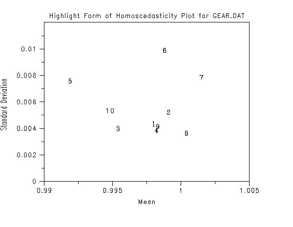
char 1 2 3 4 5 6 7 8 9 10
title Highlight Form of Homoscedasticity Plot for GEAR.DAT
highlight homoscedasticity plot y x
.
.  Different Statistics
.
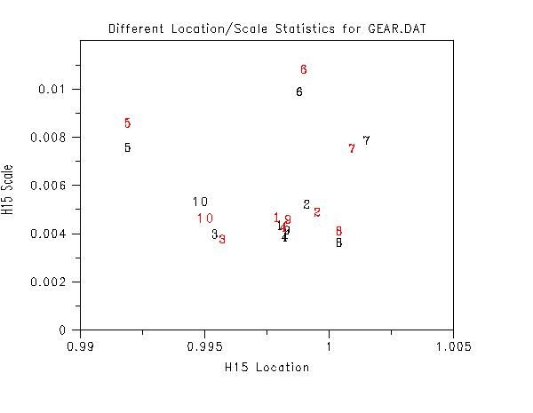
title Different Location/Scale Statistics for GEAR.DAT
label
yminimum 0
subset homoscedasticity plot y x
pre-erase off
set homo plot location h15
set homo plot scale    h15
x1label H15 Location
y1label H15 Scale
char color red all
subset homoscedasticity plot y x
pre-erase on
    

 
skip 25
read ripken.dat  y x1 to x4
.
title case asis
label case asis
x1label Mean
y1label Standard Deviation
line blank all
.
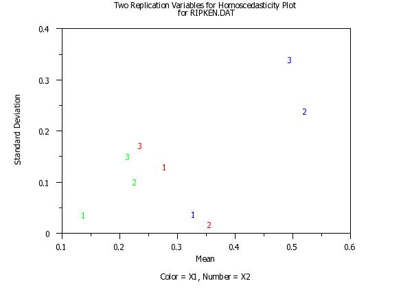
char 1 2 3 1 2 3 1 2 3
char color red red red blue blue blue green green green
x3label Color = X1, Number = X2
title Two Replication Variables for Homoscedasticity Plotcr() ...
for RIPKEN.DAT
homoscedasticity plot y x1 to x2
    

 
SKIP 25
READ MONTGOME.DAT Y1 Y2 Y3
.
title case asis
label case asis
x1label Mean
y1label Standard Deviation
line blank all
.
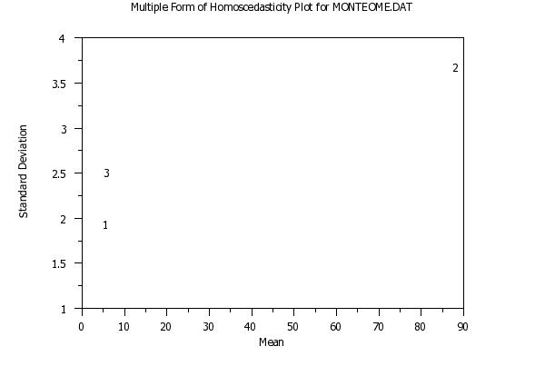
char 1 2 3
title Multiple Form of Homoscedasticity Plot for MONTEOME.DAT
multiple homoscedasticity plot y1 y2 y3
    

 
skip 25
read gear.dat  y x
.
title case asis
label case asis
x1label Mean
y1label Standard Deviation
line blank all
.
char blank blank blank 1 2 3 4 5 6 7 8 9 10
line solid dash dotted
title Highlight Form of Homoscedasticity Plot with Contour Linescr() ...
for GEAR.DAT
.
xlimits 0.99 1.005
ylimits 0  0.015
set homo plot circle technique on
pre-sort off
highlight homoscedasticity plot y x
pre-sort on
    

 
skip 25
read antibody.dat lab  ymean  ysd  nrepl
.
title case asis
label case asis
x1label Mean
y1label Standard Deviation
.
char 1 2 3 4 5 6 7 8 9 10 11 12 13 14 15 16 17 18 ...
     19 20 21 22 23 24 25
line blank all
.
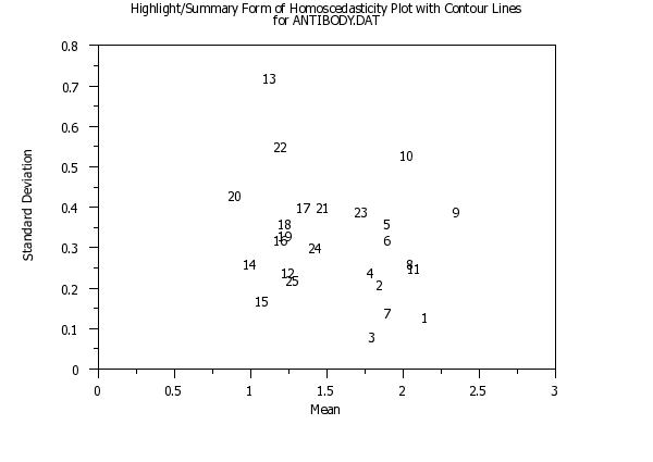
title Highlight/Summary Form of Homoscedasticity Plot with Contour Linescr() ...
for ANTIBODY.DAT
highlight summary homoscedasticity plot ymean ysd
.
char blank blank blank 1 2 3 4 5 6 7 8 9 10 11 12 13 14 15 16 17 18 ...
     19 20 21 22 23 24 25
line blank all
line solid dash dotted
xlimits 0.8  2.5
ylimits 0    1.6
.
title Highlight/Summary Form of Homoscedasticity Plot with Contour Linescr() ...
for ANTIBODY.DAT
set homo plot circle technique on
highlight summary homoscedasticity plot ymean ysd nrepl