SED navigation bar go to SED home page go to Dataplot home page go to NIST home page SED Home Page SED Staff SED Projects SED Products and Publications Search SED Pages
Dataplot Vol 1 Auxiliary Chapter

KS PLOT

Name:
    ... KS PLOT
Type:
    Graphics Command
Purpose:
    Generates a Kolmogorov-Smirnov plot.
Description:
    The Kolmogorov-Smirnov (or KS) plot is a variant of the ppcc plot. A ppcc plot is a graphical data analysis technique for determining that member of the specified distributional family which provides a "best" distributional fit to the data. The ppcc plot is based on the following two ideas:

    1. The "straightness" of the probability plot is a good measure of distributional fit. That is, the "best" distributional fit is the one with the most linear probability plot.

    2. The correlation coefficient of the points on the probabability plot is a good measure of the "straightness" (i.e., linearity) of the probability plot.

    The KS plot modifies the ppcc plot by using the value of the Kolmogorov-Smirnov goodness of fit statistic as the measure of distributional fit rather than the correlation coefficient of the probability plot. For the KS plot, we are looking for the value of the shape parameter that minimizes the Kolmogorov-Smirnov statistic.

    The KS plot is formed by selecting a value of the shape parameter and computing the value of the Kolmogorov-Smirnov goodness of fit test. The KS plot then consists of:

      Vertical axis = Kolmogorov-Smirnov goodness of fit value for the given value of the shape parameter;
      Horizontal axis = distributional family parameter value (i.e., the value of the shape parameter.

    The value of the distributional parameter (on the horizontal axis) which corresponds to the minimum of the KS plot curve (on the vertical axis) indicates the best-fit member of the family.

    One complication of the KS plot is that it is not invariant to the choice of location and scale parameters. There are two possible solutions to this.

    1. By default, the KS plot will generate a probability plot for each value of the shape parameter. It will then use the intercept and slope of the line fitted to the probability plot as the estimates of location and scale.

      For distributions that are bounded (e.g., X has to be positive), these intial estimates may be tweaked in order to obtain values of location and scale that result in the data being in an acceptable domain of the' distribution.

    2. You can specify the desired values of the location and scale parameters by entering the commands

        LET KSLOC = <value>
        LET KSSCALE = <value>

      In this case, the KS plot will execute significantly faster since it does not have to generate a probability plot for each value of the shape parameter.

    The KS plot can be used with distributions that have two shape parameters. Dataplot supports two formats for the KS plot with two shape parameters:

    1. As in the one shape parameter case, the Y axis contains the value of the KS statistic. The X axis contains the value of the second shape parameter. Each value of the first shape parameter are represented by a separate trace (i.e., curve) on the plot.

    2. Alternatively, you can generate a 3D wireframe plot.

    You can specify which format to use with the command

      SET PPCC FORMAT <TRACE/3D>

    KS plots are available for the following continuous distributional families (with the distributional parameter in parentheses) with one shape parameter:

    1. Weibull (gamma)
    2. double weibull (gamma)
    3. inverted weibull (gamma)
    4. gamma (gamma)
    5. double gamma (gamma)
    6. log gamma (gamma)
    7. inverted gamma (gamma)
    8. Wald (gamma)
    9. fatigue life (gamma)
    10. Pareto (gamma)
    11. Pareto second kind (gamma)
    12. extreme value type 2 (gamma)
    13. geometric extreme exponential (gamma)
    14. Tukey lambda (lambda)
    15. skew normal (lambda)
    16. t (nu)
    17. folded t (nu)
    18. chi-squared (nu)
    19. chi (nu)
    20. generalized logistic (alpha)
    21. log double exponential (alpha)
    22. error (alpha)
    23. lognormal (sd)
    24. power-normal (p)
    25. Von Mises (b)
    26. reciprocal (b)
    27. log-logistic (delta)
    28. Bradford (beta)

    KS plots are available for the following continuous distributional families (with the distributional parameter in parentheses) with two shape parameters:

    1. inverse Gaussian (mu, gamma)
    2. reciprocal inverse gaussian (mu,gamma)
    3. generalized gamma (gamma, c)
    4. exponentiated Weibull (gamma, theta)
    5. Beta (alpha, beta)
    6. two-sided power (n, theta)
    7. Johnson SU (alpha1, alpha2)
    8. Johnson SB (alpha1, alpha2)
    9. alpha (alpha1, alpha2)
    10. Gompertz (c, b)
    11. g and h (h, g)
    12. F (nu1, nu2)
    13. log skew normal (lambda, sd)
    14. power lognormal (nu, sd)
    15. folded normal (mu, sd)
    16. folded Cauchy (loc, scale)
    17. skew t (nu, lambda)
    18. noncentral t (nu, lambda)
    19. noncentral chi-square (nu, lambda)

    Note that if the two shape parameter case is drawn as multiple traces on a 2d plot, the value of the second shape parameter listed is represented by x axis while each curve represents a different value of the first shape parameter listed above).

    KS plots are available for the following discrete distributional families (with the distributional parameter in parentheses):

    1. geometric (p)
    2. Yule (p)
    3. Poisson (lambda)
    4. logarithmic series (theta)
    5. Hermite (alpha, beta)
    6. beta-binomial (alpha, beta, N is the sample size)
    7. negative binomial (k, p)
    8. Waring (c, a, restricted to a >= 1)

    Note that the Kolmogorov-Smirnov goodness of fit test is undefined for discrete distribution. So for discrete distributions, the chi-square goodness of fit statistic is used.

    At this point we have done limited testing of the KS plot relative to the ppcc plot. However, some preliminary simulations suggest the following:

    1. For continuous distributions with one shape parameter, the KS plot and ppcc plot both generate reasonable results for most supported distributions. Neither method demonstrates a clear advantage over the other.

    2. For continuous distributions with two shape parameters, the KS plot seems to work better than the ppcc plot.

    3. For discrete distributions, the KS plot generates smoother plots than the ppcc plot.

    In summary, either the ppcc plot and ks plot should work well for continuous distributions with a single shape parameter. However, for continuous distributions with two shape parameters or for discrete distributions, the ks plot may provide better fits.

Syntax 1:
    <family> KS PLOT <x>             <SUBSET/EXCEPT/FOR/qualification>
    where <x> is the variable of raw data values under analysis;
                <family> is one of the distributions listed above:
        WEIBULL
        DOUBLE WEIBULL
        INVERTED WEIBULL
        GAMMA
        DOUBLE GAMMA
        LOG GAMMA
        INVERTED GAMMA
        WALD
        FATIGUE LIFE
        PARETO
        PARETO SECOND KIND
        FRECHET (for extreme value type 2)
        GENERALIZED EXTREME VALUE
        GEOMETRIC EXTREME EXPONENTIAL
        TUKEY LAMBDA
        SKEW NORMAL
        T
        FOLDED T
        CHI-SQUARE
        CHI
        GENERALIZED LOGISTIC
        LOG DOUBLE EXPONENTIAL
        ERROR
        LOGNORMAL
        POWER NORMAL
        VON MISES
        RECIPROCAL
        LOG LOGISTIC
        INVERSE GAUSSIAN
        RECIPROCAL INVERSE GAUSSIAN
        GENERALIZED GAMMA
        EXPONENTIATED WEIBULL
        EXPONENTIAL POWER
        BETA
        TWO SIDED POWER
        JOHNSON SU
        JOHNSON SB
        ALPHA
        GOMPERTZ
        G AND H
        F
        LOG SKEW NORMAL
        POWER LOGNORMAL
        FOLDED NORMAL
        FOLDED CAUCHY
        SKEW T
        NONCENTRAL T
        GEOMTRIC
        YULE
        POISSON
        LOGARITHMIC SERIES
        HERMITE
        BETA BINOMIAL
        NEGATIVE BINOMIAL
        WARING

    and where the is optional.

    This syntax is used for the case where have raw data.

Syntax 2:
    <family> KS PLOT <y> <x>             <SUBSET/EXCEPT/FOR/qualification>
    where <y> is the variable of pre-computed frequencies;
                <x> is the variable of distinct values for the variable under analysis;
                <family> is one of the families listed above;
    and where the is optional.

    This syntax is used for the case where we have frequency data.

    Note: Currently, the KS plot for the case of two shape parameters or discrete distributions is not implemented for the case where the data is given in frequency format.

Examples:
    LAMBDA KS PLOT X
    T KS PLOT X
    EXTREME VALUE TYPE 2 KS PLOT X
    POISSON KS PLOT X
    LAMBDA KS PLOT F X
Note:
    The KS and ppcc plot have several attractive features for fitting.

    1. These methods have general applicability. Basically, if you can generate the percent point and cumulative distribution functions for a distribution, it is possible to generate KS and ppcc plots (the ppcc plot only requires the percent point function).

    2. When used with the probability plot, these methods provide a convenient method for obtaining estimates for location and scale. Maximum likelihood methods can at times have numerical difficulties when estimates for location or scale parameters are needed.

    3. The graphical form of these plots can show itervals of the shape parameter that are likely to generate reasonable results.

    Some disadvantages of these methods are:

    1. If the percent point function (or cumulative distribution) is expensive or difficult to compute, these methods can become impractical. If the functions have relatively simple closed forms, then these plots can be quite fast even for relatively large data sets.

    2. These plots do not generate explicit interval estimates for the estimated parameters. The plots can show reasonable neighborhoods for the shape parameters, but they do not return explicit confidence interals.

    3. These plots work best for the case with one shape parameter. They can be reasonably extended to the case with two shape parameters (although the amount of computing required is more likely to be an issue). However, they do not reasonably extend to more than two shape parameters.
Note:
    The range of parameter is determined automatically. However, if you wish to restrict the range, you can specify the lower and upper limits by appending a 1 or 2 to the parameter name and assigning a value. For example, to restrict a Weibull KS plot to values between 0.5 and 20, do the following:

      SET MINMAX 1
      LET GAMMA1 = 0.5
      LET GAMMA2 = 20
      WEIBULL KS PLOT Y

    A common use of this is to obtain a refinement of the estimate of the shape parameter. That is, an initial iteration (typically just the default values of the parameter) is used to identify the appropriate neighborhood of the optimal value of the shape parameter. Then a second iteration of the KS PLOT is generated with the parameter restricted to a much narrower range of values. Although this iteration can be repeated as many times as you like, for practical purposes a two iterations is typically sufficient.

Note:
    The KS PLOT automatically saves several parameters. The MINKS parameter contains the minimum KS goodness of fit statistic that was computed and the SHAPE parameter contains the value of the estimated distributional parameter (e.g., GAMMA for the Weibull distribution) that corresponds to MAXPPCC. The values of KSLOCS and KSSCALES will contain the estimates of location and scale for the optimal value of the shape parameter.

    In the case of two shape parameters, these are saved as SHAPE1 and SHAPE2.

Note:
    For the truncated exponential distribution, we assume that the truncation parameter, X0, is known. To set this value, enter

      LET X0 = <value>

    before generating the ppcc plot.

    For the noncentral t and noncentral chi-square distributions, we can fix the value of the degrees of freedom parameter to a single value. In this case, the ppcc plot reverts to a one shape parameter plot. Enter the commands

      LET NU1 = <value>
      LET NU2 = <value>

    where is the same for NU1 and NU2.

Note:
    The SET MINMAX command can be used to specify a minimum or maximum Weibull distribution. A value of 1 specifies a maximum Weibull distribution and a value of 2 specifies a minimum Weibull distribution.
Default:
    None
Synonyms:
    KOLMOGOROV SMIRNOV PLOT is a synonm for KS PLOT.

    FRECHET and EV2 are synonyms for EXTREME VALUE TYPE 2.

    LAMBDA KS PLOT and TUKEY KS PLOT are synonyms for TUKEY LAMBDA KS PLOT.

    STUDENT T KS PLOT is a synonym for T KS PLOT.

    The CHISQUARE term can be specified as CHISQUARE or CHI SQUARE.

    FL KS PLOT, BRIN SAUNDERS KS PLOT, and SAUNDERS BRIN are synonyms for FATIGUE LIFE KS PLOT.

    IG KS PLOT is a synonym for INVERSE GAUSSIAN KS PLOT.

    RIG KS PLOT is a synonym for RECIPROCAL INVERSE GAUSSIAN PPCC PLOT.

    GEP KS PLOT and GP KS PLOT are synonyums for GENERALIZED PARETO PLOT.

    LOGNORMAL KS PLOT and LOG-NORMAL KS PLOT are synonyms for LOG NORMAL KS PLOT.

    POWER LOG-NORMAL KS PLOT and POWER LOGNORMAL KS PLOT are synonyms for POWER LOG NORMAL KS PLOT.

    VONMISES KS PLOT and VON-MISES KS PLOT are synonyms for VON MISES KS PLOT.

    LOGLOGISTIC KS PLOT and LOG-LOGISTIC KS PLOT are synonyms for LOG LOGISTIC KS PLOT.

Related Commands: Reference:
    James J. Filliben (1975), "The Probability Plot Correlation Coefficient Test for Normality," Technometrics, Vol. 17, No. 1.

    Conover (1999), "Practical Nonparametric Statistics," Third Edition, Wiley, chapter 6.

Applications:
    Distributional Modeling
Implementation Date:
    2004/5
Program 1:
    LET NU = 10
    LET LAMBDA = 1.4
    LET Y = NONCENTRAL T RAND NUMBERS FOR I = 1 1 100
    .
    CASE ASIS
    LABEL CASE ASIS
    TITLE CASE ASIS
    X1LABEL DISPLACEMENT 6
    TITLE KS PLOTCR()(Curves Represent Different Values of NU)
    Y1LABEL Value of KS Statistic
    X1LABEL Value of LAMBDA Parameter
    NONCENTRAL T KS PLOT Y
    .
    LINE DASH
    DRAWDATA 0 0.134 10 0.134
    JUSTIFICATION CENTER
    MOVE 50 7
    TEXT NU = ^SHAPE1, LAMBDA = ^SHAPE2
    MOVE 50 4
    TEXT Location = ^KSLOCS, Scale = ^KSSCALES
    MOVE 50 1
    TEXT Minimum Value of KS Statistic = ^MINKS
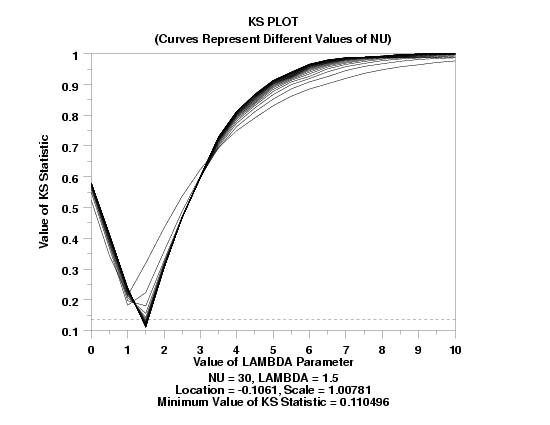
        
    plot generated by sample program

Program 2:
     
    LET THETA = 0.7
    LET Y = LOGARITHMIC SERIES RAND NUMBERS FOR I = 1 1 100
    LET THETA1 = 0.3
    LET THETA2 = 0.9
    X1LABEL THETA
    Y1LABEL CHI-SQUARE STATISTIC
    LOGARITHMIC SERIES KS PLOT Y
    JUSTIFICATION CENTER
    MOVE 50 5
    TEXT THETA = ^SHAPE
    MOVE 50 1
    TEXT Minimum Value of Chi-Square Statistic = ^MINKS
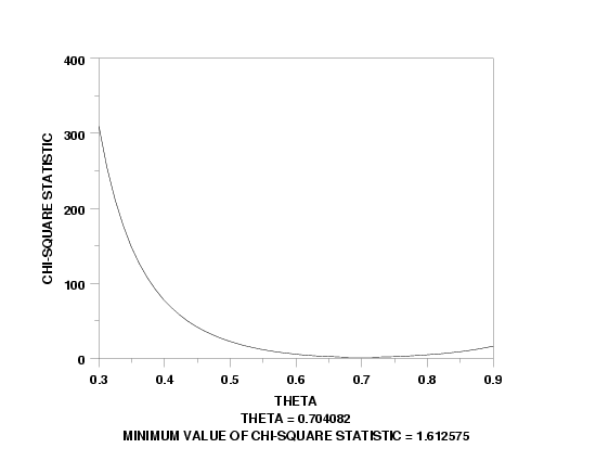
        
    plot generated by sample program

Privacy Policy/Security Notice
Disclaimer | FOIA

NIST is an agency of the U.S. Commerce Department.

Date created: 05/24/2004
Last updated: 05/12/2016

Please email comments on this WWW page to alan.heckert@nist.gov.