
|
BBNPDFName:
 , ,
 , and
and N. , and
and N.
 and
and  ,
the resulting distribution is referred to as a beta-binomial
distribution. For a standard binomial distribution, p
is assumed to be fixed for successive trials. For the
beta-binomial distribution, the value of p changes
for each trial. ,
the resulting distribution is referred to as a beta-binomial
distribution. For a standard binomial distribution, p
is assumed to be fixed for successive trials. For the
beta-binomial distribution, the value of p changes
for each trial.
The beta-binomial distribution has the following probability mass function:

where B is the complete beta
function and
Note that some sources reverse the role of

<SUBSET/EXCEPT/FOR qualification> where <x> is a number, parameter, or variable containing non-negative integer values; <alpha> is a number, parameter, or variable that specifies the first shape parameter; <beta> is a number, parameter, or variable that specifies the second shape parameter; <n> is a number, parameter, or variable that specifies the third shape parameter; <y> is a variable or a parameter (depending on what <x> is) where the computed beta-binomial pdf value is stored; and where the <SUBSET/EXCEPT/FOR qualification> is optional.
LET A = BBNPDF(X,2.1,4,N) LET X2 = BBNPDF(X1,ALPHA,BETA,N)
Alternatively, it can be derived from the Polya urn model for contagion. An urn containing w white balls and b black balls is augmented after each draw of a single ball by c balls of the drawn color (the ball withdrawn is also replaced). X is the total number of white balls drawn after n draws. This is known as the Polya distribution with probability mass function
This probability mass function can also be given in the following equivalent forms (given on page 245 of Johnson, Kotz, and Kemp).
or
The Polya distribution is somewhat more general than the beta-binomial in that the w, b, and c parameters are not restricted to positive numbers. Johnson, Kotz, and Kemp also point out the following special cases of the Polya distribution based on the sign of c.
The forms given here only support the case where w/c and b/c are positive (i.e., the beta-binomial or negative hypergeometric cases). Be aware that there are a number of derivations and formulas for the probability mass function for this distribution in the literature. It may be referred to as the inverse hypergeometric distribution, the hypergeometric waiting-time distribution, the Markov-Polya distribution, or the generalized hypergeometric distribution.
LET ALPHA = <value> LET BETA = <value> LET Y = BETA BINOMIAL RANDOM NUMBERS FOR I = 1 1 N
BETA BINOMIAL PROBABILITY PLOT Y
BETA BINOMIAL CHI-SQUARE GOODNESS OF FIT Y
To obtain the maximum likelihood estimates of
Dataplot computes the maximum likelihood estimates using
Applied Statistics algorithm 189 written by David Smith
(see References below). Note that the Smith algorithm
computes the maximum likelihood estimates for the
beta-binomial distribution in terms of the parameters

Dataplot prints the estimates for both parameterizations.
You can generate estimates of
LET ALPHA1 = <value> LET ALPHA2 = <value> LET BETA1 = <value> LET BETA2 = <value> BETA BINOMIAL KS PLOT Y BETA BINOMIAL KS PLOT Y2 X2 BETA BINOMIAL KS PLOT Y3 XLOW XHIGH BETA BINOMIAL PPCC PLOT Y BETA BINOMIAL PPCC PLOT Y2 X2 BETA BINOMIAL PPCC PLOT Y3 XLOW XHIGH The default values of alpha1 and alpha2 are 0.5 and 5, respectively. The default values for beta1 and beta2 are 0.5 and 5, respectively. Due to the discrete nature of the percent point function for discrete distributions, the ppcc plot will not be smooth. For that reason, if there is sufficient sample size the KS PLOT (i.e., the minimum chi-square value) is typically preferred. However, it may sometimes be useful to perform one iteration of the PPCC PLOT to obtain a rough idea of an appropriate neighborhood for the shape parameters since the minimum chi-square statistic can generate extremely large values for non-optimal values of the shape parameters. Also, since the data is integer values, one of the binned forms is preferred for these commands.
"Statistical Distributions", 2nd Edition, Evans, Hastings, and Peacock, 1994 (chapter 5). "Algorithm AS 189: Maximum Likelihood Estimation of the Parameters of the Beta Binomial Distribution", D. M. Smith, Applied Statistics, 1983, Vol. 32, No. 2.
XLIMITS 0 50
XTIC OFFSET 0.5 0.5
LINE BLANK
SPIKE ON
SPIKE THICKNESS 0.3
.
TITLE CASE ASIS
LABEL CASE ASIS
X1LABEL Number of Successes
Y1LABEL Probability Mass
TITLE DISPLACEMENT 2
Y1LABEL DISPLACEMENT 15
X1LABEL DISPLACEMENT 12
.
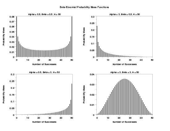
MULTIPLOT 2 2
MULTIPLOT CORNER COORDINATES 0 0 100 95
MULTIPLOT SCALE FACTOR 2
.
TITLE Alpha = 0.5, Beta = 0.5, N = 50
PLOT BBNPDF(X,0.5,0.5,50) FOR X = 0 1 50
.
TITLE Alpha = 3, Beta = 0.5, N = 50
PLOT BBNPDF(X,3.0,0.5,50) FOR X = 0 1 50
.
TITLE Alpha = 0.5, Beta = 3, N = 50
PLOT BBNPDF(X,0.5,3.0,50) FOR X = 0 1 50
.
TITLE Alpha = 3, Beta = 3, N = 50
PLOT BBNPDF(X,3.0,3.0,50) FOR X = 0 1 50
.
END OF MULTIPLOT
.
CASE ASIS
JUSTIFICATION CENTER
MOVE 50 97
TEXT Beta-Binomial Probability Mass Functions

Date created: 8/23/2006 |