BIPLOT

BIPLOT (LET)

Let Subcommand

Compute the biplot of a matrix.

Given a matrix X where the columns denote variables and the rows denote observations, the biplot can be used to generate a graphical representation of X. The "bi" in biplot refers to the joint representation of the rows and columns of X, not the fact that the biplot is typically rendered as a two-dimensional plot.

The primary purpose of the biplot is to determine what type of model might be appropriate for analyzing the data in the matrix.

The biplot method used in Dataplot is based on the singular value factorization of the matrix. The rank 2 singular value factorization leads to the following equation (X is a matrix with n rows and p columns)

\( X_{2} = A B' \)

where

\( A = \left( \begin{array}{ll} U_{11} l_{1}^{k} & U_{12} l_{2}^{k} \\ U_{21} l_{1}^{k} & U_{22} l_{2}^{k} \\ \cdots & \cdots \\ U_{n1} l_{1}^{k} & U_{n2} l_{2}^{k} \\ \end{array} \right) \)



\( B' = \left( \begin{array}{llcl} V_{11} l_{1}^{1-k} & V_{21} l_{1}^{1-k} & \cdots & V_{p1} l_{1}^{1-k} \\ V_{21} l_{2}^{1-k} & V_{22} l_{2}^{1-k} & \cdots & V_{p2} l_{2}^{1-k} \\ \end{array} \right) \)



\( l_1 \ge l_2 \ge \cdots \ge l_p \) are the eigenvalues of X
U are the left eigenvectors of X
V are the right eigenvectors of X


The rank 2 approximation will be useful if the \( l_3 \cdots l_p \) are small relative to the \( l_1 \) and \( l_2 \).

The two colums of A are used as coordinates for plotting the n rows (these are referred to as the row markers). Similarly, the two rows of B' are the coordinates for plotting the variables (these are referred to as the column markers).

The following values of k are typically used:

k = 0.5	when row and column markers are jointly displayed
k = 0	when only column markers are displayed
k = 1	when only row markers are displayed

To set the value of k, enter the command

SET BIPLOT COEFFICIENT <VALUE>

The default is 0.5 (for versions prior to 2018/11, the default is 1.0). Values outside the (0,1) interval will be set to the default.

It is also common to scale the data by subtracting the column mean. Alternatively, you can subtract the grand mean. To specify the scaling to use, enter

SET BIPLOT SCALE <COLUMN MEAN/GRAND MEAN/NONE>

The default is COLUMN MEAN (for versions prior to 2018/11, the default is GRAND MEAN).

Although the rank 2 singular value factorization is most commonly used for biplots, the biplot can in fact be based on any rank 2 approximation of the X matrix. However, other rank 2 approximations are not currently supported in Dataplot.

A goodness of fit measure for the biplot is

\( \frac{l_1 + l_2} {l_1 + l_2 + l_3 + \cdots + l_p} \)

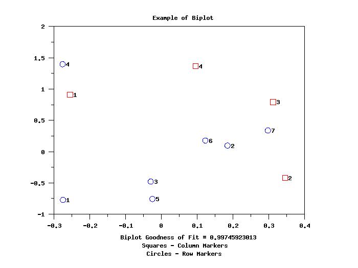
This is the ratio of the sum of the first two eigenvalues to the sum of all the eigenvalues. This value is an indication of how well the rank 2 approximation of X fits the original X matrix.

Dataplot saves this goodness of fit statistic in the parameter BIPLOTGF when it executes the BIPLOT command.

The primary application of the biplot is as a diagnostic tool. Specifically,

1. If both the row markers and column markers are colinear and they form a 90 degree angle, an additive model is suggested.

2. If both the row markers and column markers are colinear but they do not form a 90 degree angle, a concurrent model is suggested.

3. If the row markers are colinear but the column markers are not colinear, a column linear model is suggested.

4. If the row markers are not colinear but the column markers are colinear, a row linear model is suggested.

For a disucussion of row linear, column linear, and concurrent models, see the Mandel reference. For a fuller discussion of interpreting and using biplots, see the References section below.

LET <y> <x> <tag> = BIPLOT <m>
            <SUBSET/EXCEPT/FOR qualification>
            where <m> is a matrix for which the biplot coordinates are to be computed;
            <y> is an variable where the y coordinates of the biplot values are saved;
            <x> is an variable where the x coordinates of the biplot values are saved;
            <tag> is a variable that identifies whether the given row of <y> and <x> is a row marker (<tag> = 1) or a column marker (<tag> = 2);
and where the <SUBSET/EXCEPT/FOR qualification> is optional.

LET Y X TAG = BIPLOT M

Dataplot generates the most basic form of the biplot. The Gower, Lubbe, and le Roux (2011) book provides an extensive treatment of the many variants of the basic biplot.

In the terminology of Gower, Lubbe, and le Roux, Dataplot generates a 2-dimensional principal components analysis (PCA) asymmetric biplot. Asymmetric implies the rows and columns of the matrix cannot be interchanged. The columns represent continuous variables. Coordinates are generated in 2 dimensions and the rank 2 approximation is based on the singular value factorization.

Mandel (1995) discusses "row linear" and "column linear" models for two-way tables. This is an alternative to the use of biplots. Mandel gives some comparisons of his models to the biplot. Row linear and column linear models are what Gabriel refers to as "row regressions" and "column regressions".

Matrices are created with either the READ MATRIX command or the MATRIX DEFINITION command.

The columns of a matrix are accessible as variables by appending an index to the matrix name. For example, the 4x4 matrix C has columns C1, C2, C3, and C4. These columns can be operated on like any other Dataplot variable.

The maximum size matrix that Dataplot can handle is set when Dataplot is built on a particular site. However, for the size problems for which biplots are used, insufficient storage space for the matrix is typically not an issue.

None

None

READ MATRIX	=	Read data into a matrix.
PRINCIPAL COMPONENTS	=	Compute the principal components of a matrix.
SINGULAR VALUES	=	Compute the singular values of a matrix.
SINGULAR VALUE FACTORIZATION	=	Compute the singular value factorization of a matrix.
TWO WAY PLOT	=	Given a response variable and associated variables containing laboratory id's and material id's, generate a plot of each laboratory against the column average. In addition, perform a row linear (or column linear) analysis of variance.

Gabriel and Badru (1978), "The biplot as a diagnostic tool for models of two-way tables," Technometrics, Vol. 20, pp. 47-68.

du Toit, Steyn, and Stumpf (1986), "Graphical Exploratory Data Analysis," Springer-Verlang, 1986, pp. 107-114.

Mandel (1995), "Analysis of Two-Way Layouts," Chapman-Hall, pp. 49-53.

Gower, Lubbe, Le Roux (2011), "Understanding Biplots", Wiley.

Multivariate Analysis, Analysis of Two-Way Tables

2009/04
2018/11: Change the default for SET BIPLOT COEFFICIENT
2018/11: Change the default for SET BIPLOT SCALING

 
.  Step 1: Define data
.
.          Source: "The Biplot as a Diagnostic Tool for Models of
.                  Two-Way Tables", Brandu, Gabriel, Technometrics,
.                  February, 1978.
.
.                  Data is yeilds of cotton, with rows denoting variety
.                  and columns denoting center.
.
DIMENSION 100 COLUMNS
READ MATRIX M
 1.55 1.26 1.41  1.78
 3.39 3.47 2.82  3.89
 1.95 1.91 1.74  2.29
10.47 9.12 9.55 17.78
 1.45 1.51 1.41  1.70
 3.72 3.55 3.09  4.27
 4.47 4.07 3.98  4.47
END OF DATA
.
LET P = MATRIX NUMBER OF COLUMNS M
LOOP FOR K = 1 1 P
    LET M^K = LOG(M^K)
END OF LOOP
.
.  Step 2: Generate the coordinates for the biplot (this is a
.          combined row/column marker biplot).
.
LET Y X TAG = BIPLOT M
LET Y2 = Y
LET X2 = -X
.
.  Step 3: Now plot the biplot.
.
.
.  Step 3a: Iteration 1 will draw row markers as filled
.           circle and column markers as filled squares.
.
TITLE Example of Biplot
TITLE OFFSET 2
TITLE CASE AS IS
LABEL CASE ASIS
X1LABEL Biplot Goodness of Fit = ^BIPLOTGF
LEGEND CASE ASIS
LEGEND JUSTIFICATION CENTER
LEGEND 1 Squares - Column Markers
LEGEND 2 Circles - Row Markers
LEGEND 1 COORDINATES 50 7
LEGEND 2 COORDINATES 50 4
.
CHARACTER HW 2.0 1.5 ALL
CHARACTER CIRCLE SQUARE
CHARACTER FILL SOLID ALL
CHARACTER COLOR BLUE RED
LINE BLANK ALL
PLOT Y2 X2 TAG
.
.  Step 3b: Now generate row and column ID's
.
LEGEND 1
LEGEND 2
LIMITS FREEZE
PRE-ERASE OFF
CHARACTER OFFSET 1.5 0 ALL
CHARACTER COLOR BLACK ALL
.
LET NTOT = SIZE Y
LET ROWID = SEQUENCE 1 1 NTOT
CHARACTER AUTOMATIC ROWID
PLOT Y2 X2 ROWID SUBSET TAG = 1
PLOT Y2 X2 ROWID SUBSET TAG = 2