SED navigation bar go to SED home page go to Dataplot home page go to NIST home page SED Home Page SED Staff SED Projects SED Products and Publications Search SED Pages
Dataplot Vol 2 Vol 1

BTAPDF

Name:
    BTAPDF (LET)
Type:
    Library Function
Purpose:
    Compute the Borel-Tanner probability density function.
Description:
    Given a single queue with random arrival times of customers at constant rate l, constant service time beta, and k initial customers, the Borel-Tanner distribution is the distribution of the total number of customers served before the queue vanishes.

    The probability mass function of the Borel-Tanner distribution is

      p(x;lambda,k) = k*EXP(-lambda*x)*(lambda*x)**(x-k)/(x*(x-k)!),
   x >= k, 0 < lambda < 1

    with lambda and k denoting the shape parameters. The k shape parameter is a positive integer and lambda = l beta.

    The mean and variance of the Borel-Tanner distribution are

      mean = k/(1-lambda)
      variance = k*lambda/(1-lambda)^3
Syntax:
    LET <y> = BTAPDF(<x>,<lambda>,<k>)
                            <SUBSET/EXCEPT/FOR qualification>
    where <x> is a positive integer variable, number, or parameter;
                <lambda> is a number or parameter in the range (0,1) that specifies the first shape parameter;
                <k> is a number or parameter denoting a positive integer that specifies the first shape parameter;
                <y> is a variable or a parameter where the computed Borel-Tanner pdf value is stored;
    and where the <SUBSET/EXCEPT/FOR qualification> is optional.
Examples:
    LET A = BTAPDF(3,0.5,3)
    LET Y = BTAPDF(X1,0.3,2)
    PLOT BTAPDF(X,0.3,2) FOR X = 2 1 20
Note:
    For a number of commands utilizing the Borel-Tanner distribution, it is convenient to bin the data. There are two basic ways of binning the data.

    1. For some commands (histograms, maximum likelihood estimation), bins with equal size widths are required. This can be accomplished with the following commands:

        LET AMIN = MINIMUM Y
        LET AMAX = MAXIMUM Y
        LET AMIN2 = AMIN - 0.5
        LET AMAX2 = AMAX + 0.5
        CLASS MINIMUM AMIN2
        CLASS MAXIMUM AMAX2
        CLASS WIDTH 1
        LET Y2 X2 = BINNED

    2. For some commands, unequal width bins may be helpful. In particular, for the chi-square goodness of fit, it is typically recommended that the minimum class frequency be at least 5. In this case, it may be helpful to combine small frequencies in the tails. Unequal class width bins can be created with the commands

        LET MINSIZE = <value>
        LET Y3 XLOW XHIGH = INTEGER FREQUENCY TABLE Y

      If you already have equal width bins data, you can use the commands

        LET MINSIZE = <value>
        LET Y3 XLOW XHIGH = COMBINE FREQUENCY TABLE Y2 X2

      The MINSIZE parameter defines the minimum class frequency. The default value is 5.

Note:
    You can generate Borel-Tanner random numbers and probability plots with the following commands:

      LET N = VALUE
      LET K = <value>
      LET LAMBDA = <value>
      LET Y = BOREL-TANNER RANDOM NUMBERS FOR I = 1 1 N

      BOREL TANNER PROBABILITY PLOT Y
      BOREL TANNER PROBABILITY PLOT Y2 X2
      BOREL TANNER PROBABILITY PLOT Y3 XLOW XHIGH

    To obtain the maximum likelihood estimate of lambda assuming that k is known, enter the command

      BOREL TANNER MAXIMUM LIKELIHOOD Y
      BOREL TANNER MAXIMUM LIKELIHOOD Y2 X2

    The maximum likelihood estimate is

      lambdahat = (xbar - k)/xbar

    with xbar denoting the sample mean.

    For a given value of k, generate an estimate of lambda based on the maximum ppcc value or the minimum chi-square goodness of fit with the commands

      LET K = <value>
      LET LAMBDA1 = <value>
      LET LAMBDA2 = <value>
      BOREL TANNER KS PLOT Y
      BOREL TANNER KS PLOT Y2 X2
      BOREL TANNER KS PLOT Y3 XLOW XHIGH
      BOREL TANNER PPCC PLOT Y
      BOREL TANNER PPCC PLOT Y2 X2
      BOREL TANNER PPCC PLOT Y3 XLOW XHIGH

    The default values of LAMBDA1 and LAMBDA2 are 0.05 and 0.95, respectively. The value of k should typically be set to the minimum value of the data. Due to the discrete nature of the percent point function for discrete distributions, the ppcc plot will not be smooth. For that reason, if there is sufficient sample size the KS PLOT (i.e., the minimum chi-square value) is typically preferred. Also, since the data is integer values, one of the binned forms is preferred for these commands.

    To generate a chi-square goodness of fit test, enter the commands

      LET K = <value>
      LET LAMBDA = <value>
      BOREL-TANNER CHI-SQUARE GOODNESS OF FIT Y2 X2
      BOREL-TANNER CHI-SQUARE GOODNESS OF FIT Y3 XLOW XHIGH
Note:
    The case where k = 1 is referred to as the Borel distribution. It has probability mass function

      p(x;lambda) = (lambda*x)**(x-1)*EXP(-lambda*x)/x!
    x = 1, 2, ... ; 0 < lambda < 1
Note:
    If the Borel-Tanner distribution is shifted to start at X = 0 and is reparameterized with

      lambda = lambda
      theta = klambda

    the resulting distribution is referred to as the Lagrange-Poisson distribution (or the Consul generalized Poisson distribution). This distribution has probability mass function

      p(x;lambda,theta) = theta*(theta+x*lambda)**(x-1)*
EXP(-theta-x*lambda)/x!    x = 0, 1, ...; 0 < ;lambda < 1; theta > 0
Default:
    None
Synonyms:
    None
Related Commands:
    BTACDF = Compute the Borel-Tanner cumulative distribution function.
    BTAPPF = Compute the Borel-Tanner percent point function.
    POIPDF = Compute the Poisson probability mass function.
    HERPDF = Compute the Hermite probability mass function.
    BINPDF = Compute the binomial probability mass function.
    NBPDF = Compute the negative binomial mass density function.
    GEOPDF = Compute the geometric probability mass function.
    INTEGER FREQUENCY TABLE = Generate a frequency table at integer values with unequal bins.
    COMBINE FREQUENCY TABLE = Convert an equal width frequency table to an unequal width frequency table.
    KS PLOT = Generate a minimum chi-square plot.
    MAXIMUM LIKELIHOOD = Perform maximum likelihood estimation for a distribution.
Reference:
    Haight and Breuer (1960), "The Borel-Tanner Distribution", Biometrika, 47, pp. 143-150.

    Johnson, Kotz, and Kemp (1992), "Univariate Discrete Distributions", Second Edition, Wiley, pp. 394-396.

Applications:
    Distributional Modeling
Implementation Date:
    2006/5
Program:
     
    let k = 2
    let lambda = 0.8
    let y = borel tanner random numbers for i = 1 1 500
    .
    let y3 xlow xhigh = integer frequency table y
    class lower 1.5
    class width 1
    let amax = maximum y
    let amax2 = amax + 0.5
    class upper amax2
    let y2 x2 = binned y
    .
    let k = minimum y
    borel tanner mle y
    relative histogram y2 x2
    limits freeze
    pre-erase off
    line color blue
    plot btapdf(x,lambdaml,k) for x = 2 1 amax
    limits
    pre-erase on
    line color black
    let lambda = lambdaml
    borel tanner chi-square goodness of fit y3 xlow xhigh
    case asis
    justification center
    move 50 97
    text Lambda = ^lambdaml
    move 50 93
    text Minimum Chi-Square = ^minks, 95% CV = ^cutupp95
    .
    let k = 2
    label case asis
    x1label Lambda
    y1label Minimum Chi-Square
    let lambda1 = 0.5
    let lambda2 = 0.9
    borel tanner ks plot y3 xlow xhigh
    let lambda = shape
    borel tanner chi-square goodness of fit y3 xlow xhigh
    case asis
    justification center
    move 50 97
    text Lambda = ^lambda
    move 50 93
    text Minimum Chi-Square = ^minks, 95% CV = ^cutupp95
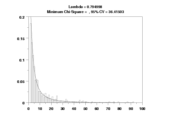
        
    plot generated by sample program
                      CHI-SQUARED GOODNESS-OF-FIT TEST
     
    NULL HYPOTHESIS H0:      DISTRIBUTION FITS THE DATA
    ALTERNATE HYPOTHESIS HA: DISTRIBUTION DOES NOT FIT THE DATA
    DISTRIBUTION:            BOREL-TANNER
     
    SAMPLE:
       NUMBER OF OBSERVATIONS      =      500
       NUMBER OF NON-EMPTY CELLS   =       27
       NUMBER OF PARAMETERS USED   =        2
     
    TEST:
    CHI-SQUARED TEST STATISTIC     =    17.10083
       DEGREES OF FREEDOM          =       24
       CHI-SQUARED CDF VALUE       =    0.155670
     
       ALPHA LEVEL         CUTOFF              CONCLUSION
               10%       33.19624               ACCEPT H0
                5%       36.41503               ACCEPT H0
                1%       42.97982               ACCEPT H0
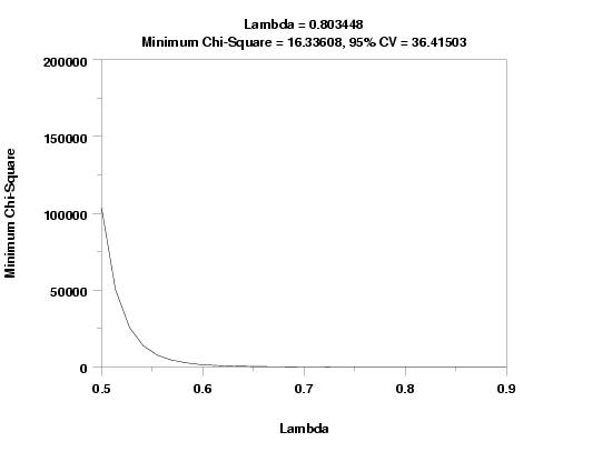
     
        
    plot generated by sample program
                      CHI-SQUARED GOODNESS-OF-FIT TEST
     
    NULL HYPOTHESIS H0:      DISTRIBUTION FITS THE DATA
    ALTERNATE HYPOTHESIS HA: DISTRIBUTION DOES NOT FIT THE DATA
    DISTRIBUTION:            BOREL-TANNER
     
    SAMPLE:
       NUMBER OF OBSERVATIONS      =      500
       NUMBER OF NON-EMPTY CELLS   =       27
       NUMBER OF PARAMETERS USED   =        2
     
    TEST:
    CHI-SQUARED TEST STATISTIC     =    16.33608
       DEGREES OF FREEDOM          =       24
       CHI-SQUARED CDF VALUE       =    0.124435
     
       ALPHA LEVEL         CUTOFF              CONCLUSION
               10%       33.19624               ACCEPT H0
                5%       36.41503               ACCEPT H0
                1%       42.97982               ACCEPT H0


Date created: 6/5/2006
Last updated: 6/5/2006
Please email comments on this WWW page to alan.heckert@nist.gov.