EMPIRICAL QUANTILE FUNCTION

EMPIRICAL QUANTILE FUNCTION (LET)

Let Subcommand

Compute the empirical quantile function.

The quantile function is the inverse of the cumulative distribution function, F,
\( Q(u) = F^{-1}(u) \hspace{0.2in} 0 < u < 1 \)

Given a set of ordered data, x₁ ≤ x₂ ... ≤ x_n, an empirical estimate of the quantile function can be obtained from the following piecewise linear function

\( \hat{Q}(u) = (nu - j + \frac{1}{2}) x_{(j+1)} + (j + \frac{1}{2} - nu) x_{j} \)

\( \frac{2j - 1}{2n} \le u \le \frac{2j + 1}{2n} \)

This will be computed for a specified number of equi-spaced points between the lower and upper limits. Dataplot will use the number of points in the sample if this is greater than 1,000. Otherwise 1,000 points will be used.

LET <y> <u> = EMPIRICAL QUANTILE FUNCTION <x>
                        <SUBSET/EXCEPT/FOR qualification>
where <x> is the response variable;
            <y> is a variable containing the empirical quantile function;
<u> is a variable containing the values where the empirical quantile function is computed;
and where the <SUBSET/EXCEPT/FOR qualification> is optional.

LET Y U = EMPIRICAL QUANTILE FUNCTION X
LET Y U = EMPIRICAL QUANTILE FUNCTION X SUBSET X > 0

None

None

EMPIRICAL QUANTILE PLOT	=	Generate an empirical quantile plot.
EMPIRICAL CDF PLOT	=	Generates an empiricial CDF plot.
KAPLAN MEIER PLOT	=	Generates a Kaplan Meier plot.
PROBABILITY PLOT	=	Generates a probability plot.
INFORMATIVE QUANTILE FUNCTION	=	Compute the informative quantile function.

"MIL-HDBK-17-1F Volume 1: Guidelines for Characterization of Structural Materials", Depeartment of Defense, pp. 8-36, 8-37, 2002.

Parzen (1983), "Informative Quantile Functions and Identification of Probability Distribution Types", Technical Report No. A-26, Texas A&M University.

Distributional Analysis

2017/02

 
. Step 1:   Define some default plot control features
.
title offset 2
title case asis
case asis
label case asis
line color blue red
multiplot scale factor 2
multiplot corner coordinates 5 5 95 95
.
. Step 2:   Create 50, 100, 200, and 1000 normal random numbers and
.           compute the empirical quantile funciton
.
let nv = data 50 100 200 1000
let p = sequence 0.01 0.01 .99
let y2 = norppf(p)
.
. Step 3:   Loop through the four cases and compute and plot the
.           empirical quantile funciton with overlaid NORPPF
.
multiplot 2 2
loop for k = 1 1 4
    let n = nv(k)
    let x = norm rand numb for i = 1 1 n
    let y u = empirical quantile function x
    title N: ^n
    plot y u and
    plot y2 p
end of loop
end of multiplot
.
justification center
move 50 97
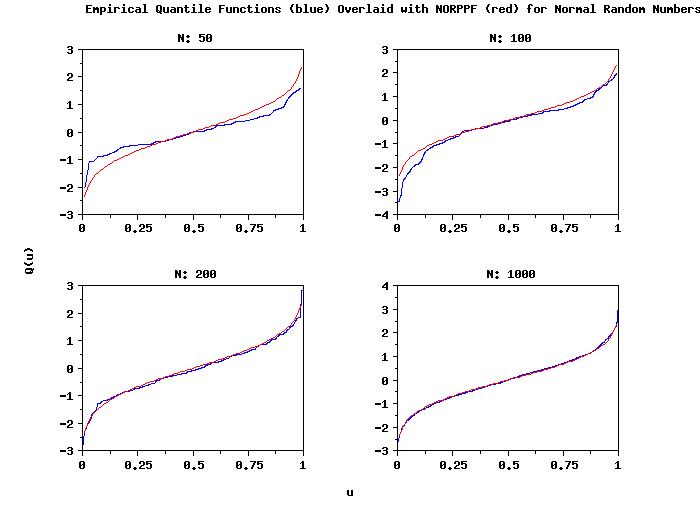
text Empirical Quantile Functions (blue) Overlaid with ...
NORPPF (red) for Normal Random Numbers
move 50 5
text u
direction vertical
move 5 50
text Q(u)