|
|
LBEPDFName:
 , ,
 ,
c, and d. ,
c, and d.
with
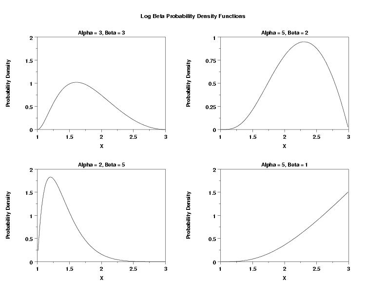
The log beta distribution has been proposed as an alternative to the log normal distribution. It has the advantage of being able to model both left and right skewness (the lognormal can only model right skewness). It may also be more appropriate when the data has an upper bound. The log beta distribution can be generalized with location and scale parameters in the usual way.
<SUBSET/EXCEPT/FOR qualification> where <x> is a number, parameter, or variable; <alpha> is a number, parameter, or variable that specifies the first shape parameter; <beta> is a number, parameter, or variable that specifies the second shape parameter; <c> is a number, parameter, or variable that specifies the third shape parameter; <d> is a number, parameter, or variable that specifies the fourth shape parameter; <loc> is a number, parameter, or variable that specifies the optional location parameter; <scale> is a number, parameter, or variable that specifies the optional scale parameter; <y> is a variable or a parameter (depending on what <x> is) where the computed log beta pdf value is stored; and where the <SUBSET/EXCEPT/FOR qualification> is optional. The location and scale parameters are optional (the default values are zero and one, respectively).
LET Y = LBEPDF(X,ALPHA,BETA,C,D) PLOT LBEPDF(X,6,6,1,3) FOR X = 1.01 0.01 2.99
LET BETA = <value> LET C = <value> LET D = <value> LET Y = LOG BETA RANDOM NUMBERS FOR I = 1 1 N LOG BETA PROBABILITY PLOT Y LOG BETA PROBABILITY PLOT Y2 X2 LOG BETA PROBABILITY PLOT Y3 XLOW XHIGH LOG BETA KOLMOGOROV SMIRNOV GOODNESS OF FIT Y LOG BETA CHI-SQUARE GOODNESS OF FIT Y2 X2 LOG BETA CHI-SQUARE GOODNESS OF FIT Y3 XLOW XHIGH The following commands can be used to estimate the alpha and beta shape parameters (the lower and upper limit parameters c and d are assumed known) for the log beta distribution:
LET D = <value> LET ALPHA1 = <value> LET ALPHA2 = <value> LET BETA1 = <value> LET BETA2 = <value> LOG BETA PPCC PLOT Y LOG BETA PPCC PLOT Y2 X2 LOG BETA PPCC PLOT Y3 XLOW XHIGH LOG BETA KS PLOT Y LOG BETA KS PLOT Y2 X2 LOG BETA KS PLOT Y3 XLOW XHIGH The default values for ALPHA1 and ALPHA2 are 0.5 and 10. The default values for BETA1 and BETA2 are 0.5 and 10. Note that the log beta percent point function is expensive to compute. For larger data samples, this can make the above fit commands slow. We can do the following to improve the speed of these commands.
title displacement 2
y1label displacement 17
x1label displacement 12
case asis
title case asis
label case asis
y1label Probability Density
x1label X
.
let c = 1
let d = 3
.
multiplot corner coordinates 0 0 100 95
multiplot scale factor 2
multiplot 2 2
.
title Alpha = 3, Beta = 3
plot lbepdf(x,3,3,c,d) for x = 1.01  0.01  2.99
.
title Alpha = 5, Beta = 2
plot lbepdf(x,5,2,c,d) for x = 1.01  0.01  2.99
.
title Alpha = 2, Beta = 5
plot lbepdf(x,2,5,c,d) for x = 1.01  0.01  2.99
.
title Alpha = 5, Beta = 1
plot lbepdf(x,5,1,c,d) for x = 1.01  0.01  2.99
.
end of multiplot
.
justification center
move 50 97
text Log Beta Probability Density Functions
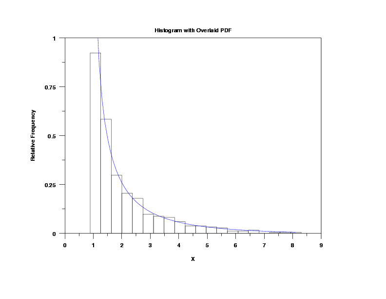
Program 2:
let alpha = 0.7
let beta = 2.1
let c = 1
let d = 10
let y = log beta rand numb for i = 1 1 500
let y2 x2 = binned y
let amin = minimum y
let amax = maximum y
.
title displacement 2
case asis
title case asis
label case asis
.
title Histogram with Overlaid PDF
y1label Relative Frequency
x1label X
relative histogram y2 x2
limits freeze
pre-erase off
line color blue
plot lbepdf(x,alpha,beta,c,d) for x = amin 0.1 amax
limits
pre-erase on
line color black
.
title Log Beta Probability Plot
y1label Theoretical
x1label Data
char x
line bl
log beta probability plot y
justification center
move 50 6
text PPCC = ^ppcc
line solid
char blank
.
multiplot corner coordinates 0 0 100 100
multiplot scale factor 2
y1label displacement 17
x1label displacement 12
multiplot 2 2
.
let alpha1 = 0.5
let alpha2 = 5
let beta1 = 0.5
let beta2 = 5
set ppcc plot data points 100
.
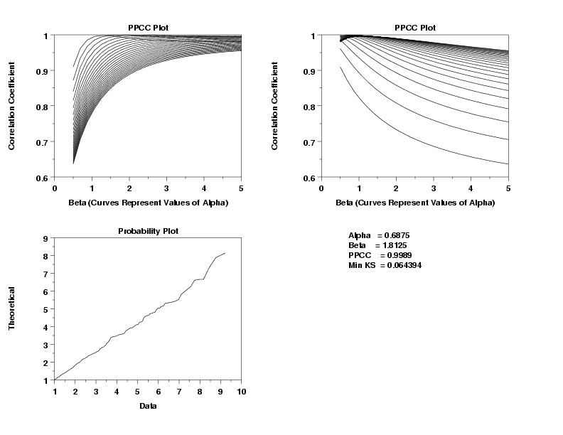
title PPCC Plot
y1label Correlation Coefficient
x1label Beta (Curves Represent Values of Alpha)
log beta ppcc plot y
let alpha = shape1
let beta = shape2
set ppcc plot axis order reverse
log beta ppcc plot y
set ppcc plot axis order default
title Probability Plot
y1label Theoretical
x1label Data
log beta probability plot y
log beta kolmogorov smirnov goodness of fit y
title
label
plot
justification left
move 25 90
text Alpha = ^alpha
move 25 85
text Beta = ^beta
move 25 80
text PPCC = ^ppcc
move 25 75
text Min KS = ^statval
end of multiplot
.
multiplot 2 2
let ksloc = 0
let ksscale = 1
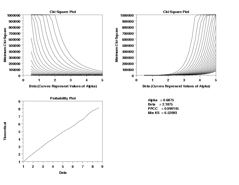
title Chi-Square Plot
y1label Minimum Chi-Square
x1label Beta (Curves Represent Values of Alpha)
log beta ks plot y2 x2
let alpha = shape1
let beta = shape2
set ppcc plot axis order reverse
log beta ks plot y2 x2
set ppcc plot axis order default
title Probability Plot
y1label Theoretical
x1label Data
log beta probability plot y2 x2
log beta chi-square goodness of fit y2 x2
title
label
plot
justification left
move 25 90
text Alpha = ^alpha
move 25 85
text Beta = ^beta
move 25 80
text PPCC = ^ppcc
move 25 75
text Min KS = ^statval
end of multiplot
Date created: 8/23/2006 |