SED navigation bar go to SED home page go to Dataplot home page go to NIST home page SED Home Page SED Staff SED Projects SED Products and Publications Search SED Pages
Dataplot Vol 2 Vol 1

QBIPDF

Name:
    QBIPDF (LET)
Type:
    Library Function
Purpose:
    Compute the quasi-binomial type I probability mass function.
Description:
    The quasi-binomial type I distribution has the following probability mass function:

      p(x;p,phi) = (m  x)*p*(p + x*phi)**(x-1)*(1-p-x*phi)**(m-x)
   x = 0, 1, 2, ..., m; 0 <= p <= 1; -p/m < phi < (1-p)/m

    with p, phi, and m denoting the shape parameters.

    The quasi-binomial type I distribution is used to model Bernoulli trials. The parameter p denotes the initial probability of success, m denotes the number of Bernoulli trials, and phi denotes how the probability of success increases or decreases with the number of successes. Specificially, when phi = 0, the quasi-binomial type I distribution reduces to the binomial distribution. When phi ≠ 0, the probability of success in the xth trial becomes

      p + x*phi
Syntax:
    LET <y> = QBIPDF(<x>,<p>,<theta>,<beta>)
                            <SUBSET/EXCEPT/FOR qualification>
    where <x> is a positive integer variable, number, or parameter;
                <p> is a number, parameter, or variable in the range (0,1) that specifies the first shape parameter;
                <phi> is a number, parameter, or variable that specifies the second shape parameter;
                <m> is a number, parameter, or variable that specifies the third shape parameter;
                <y> is a variable or a parameter (depending on what <x> is) where the computed quasi binomial type I pdf value is stored;
    and where the <SUBSET/EXCEPT/FOR qualification> is optional.
Examples:
    LET A = QBIPDF(10,0.5,0.005,20)
    LET Y = QBIPDF(X,0.7,0.01,20)
    PLOT QBIPDF(X,0.3,0.005,20) FOR X = 0 1 20
Note:
    For a number of commands utilizing the quasi binomial type I distribution, it is convenient to bin the data. There are two basic ways of binning the data.

    1. For some commands (histograms, maximum likelihood estimation), bins with equal size widths are required. This can be accomplished with the following commands:

        LET AMIN = MINIMUM Y
        LET AMAX = MAXIMUM Y
        LET AMIN2 = AMIN - 0.5
        LET AMAX2 = AMAX + 0.5
        CLASS MINIMUM AMIN2
        CLASS MAXIMUM AMAX2
        CLASS WIDTH 1
        LET Y2 X2 = BINNED

    2. For some commands, unequal width bins may be helpful. In particular, for the chi-square goodness of fit, it is typically recommended that the minimum class frequency be at least 5. In this case, it may be helpful to combine small frequencies in the tails. Unequal class width bins can be created with the commands

        LET MINSIZE = <value>
        LET Y3 XLOW XHIGH = INTEGER FREQUENCY TABLE Y

      If you already have equal width bins data, you can use the commands

        LET MINSIZE = <value>
        LET Y3 XLOW XHIGH = COMBINE FREQUENCY TABLE Y2 X2

      The MINSIZE parameter defines the minimum class frequency. The default value is 5.

Note:
    You can generate quasi-binomial type I random numbers, probability plots, and chi-square goodness of fit tests with the following commands:

      LET M = <value>
      LET P = <value>
      LET PHI = <value>
      LET Y = QUASI BINOMIAL TYPE I RANDOM NUMBERS FOR I = 1 1 N

      QUASI BINOMIAL TYPE I PROBABILITY PLOT Y
      QUASI BINOMIAL TYPE I PROBABILITY PLOT Y2 X2
      QUASI BINOMIAL TYPE I PROBABILITY PLOT Y3 XLOW XHIGH

      QUASI BINOMIAL TYPE I CHI-SQUARE GOODNESS OF FIT Y
      QUASI BINOMIAL TYPE I CHI-SQUARE GOODNESS OF FIT Y2 X2
      QUASI BINOMIAL TYPE I CHI-SQUARE ..
                              GOODNESS OF FIT Y3 XLOW XHIGH

    In fitting the quasi-binomial type I distribution to data, we typically assume that the number of trials, m, is fixed and known and we then estimate p and phi.

    To obtain the maximum likelihood estimates of p and phi, enter the command

      LET M = <value>
      QUASI BINOMIAL TYPE I MAXIMUM LIKELIHOOD Y
      QUASI BINOMIAL TYPE I MAXIMUM LIKELIHOOD Y2 X2

    For unbinned data, the maximum likelihood estimates are the solutions to the equations:

      SUM[i=1 to N][(X(i)*(X(i) - 1)/(p + X(i)*PHI) -
 SUM[i=1 to N][(M - X(i))/(1 - P - X(i)*PHI)] = 0

      SUM[i=1 to N][(m-X(i))/(1 - P - X(i)*PHI] - M*N = 0

    For binned data, the equations become

      SUM[i=1 to k][n(i)*(i-1)*i/(p+i*phi)] -
 SUM[i=1 to k][n(i)*(m-1)*i/(1-p-i*phi)] = 0

      (n/p) + SUM[i=1 to k][n(i)*(i-1)/(p+i*phi)] -
 SUM[i=1 to k][n(i)*(m-1)/(1-p-i*phi)] = 0

    with k, n, and nx denoting the number of classes, the total sample size, and the frequency of the xth class, respectively.

    These equations are known to have multiple solutions, so good starting values are required. By default, we use the starting values recommended by Consul and Famoye

      p = 1 - (f0/n)**(1/m)

      phi = (1/(2*(m-2))*(-1 + SQRT(1 + 4*(m-2)*(-1+xbar/(m*p))/(m-1)))

    with f0 denoting the frequency of the class x = 0 and xbar denoting the sample mean.

    Alternatively, you can specify your own starting values by entering the commands

      LET PSTART = <value>
      LET PHISTART = <value>

    Consul and Famoye give formulas for the Fisher information matrix (the inverse of the parameter variance-covariance matrix). They also give simplified formulas for the special cases m = 1, 2, or 3.

    You can generate estimates of p and phi based on the maximum ppcc value or the minimum chi-square goodness of fit with the commands

      LET M = <value>
      LET P1 = <value>
      LET P2 = <value>
      LET PHI1 = <value>
      LET PHI2 = <value>
      QUASI BINOMIAL TYPE I KS PLOT Y
      QUASI BINOMIAL TYPE I KS PLOT Y2 X2
      QUASI BINOMIAL TYPE I KS PLOT Y3 XLOW XHIGH
      QUASI BINOMIAL TYPE I PPCC PLOT Y
      QUASI BINOMIAL TYPE I PPCC PLOT Y2 X2
      QUASI BINOMIAL TYPE I PPCC PLOT Y3 XLOW XHIGH

    The default values of p1 and p2 are 0.05 and 0.95, respectively. The default values for phi1 and phi2 are phi1 = -p1/m and phi2 = (1-p1)/m.

    Due to the discrete nature of the percent point function for discrete distributions, the ppcc plot will not be smooth. For that reason, if there is sufficient sample size the KS PLOT (i.e., the minimum chi-square value) is typically preferred. However, it may sometimes be useful to perform one iteration of the PPCC PLOT to obtain a rough idea of an appropriate neighborhood for the shape parameters since the minimum chi-square statistic can generate extremely large values for non-optimal values of the shape parameters. Also, since the data is integer values, one of the binned forms is preferred for these commands.

Default:
    None
Synonyms:
    None
Related Commands:
    QBICDF = Compute the quasi-binomial type I cumulative distribution function.
    QBIPPF = Compute the quasi-binomial type I percent point function.
    BINPDF = Compute the binomial probability mass function.
    BBNPDF = Compute the beta-binomial probability mass function.
    NBPDF = Compute the negative binomial probability mass function.
    INTEGER FREQUENCY TABLE = Generate a frequency table at integer values with unequal bins.
    COMBINE FREQUENCY TABLE = Convert an equal width frequency table to an unequal width frequency table.
    KS PLOT = Generate a minimum chi-square plot.
    MAXIMUM LIKELIHOOD = Perform maximum likelihood estimation for a distribution.
Reference:
    Consul and Famoye (2006), "Lagrangian Probability Distribution", Birkhauser, pp. 70-80.
Applications:
    Distributional Modeling
Implementation Date:
    2006/8
Program 1:
     
    title size 3
    tic label size 3
    label size 3
    legend size 3
    height 3
    x1label displacement 12
    y1label displacement 15
    .
    multiplot corner coordinates 0 0 100 95
    multiplot scale factor 2
    label case asis
    title case asis
    case asis
    tic offset units screen
    tic offset 3 3
    title displacement 2
    y1label Probability Mass
    x1label X
    .
    ylimits 0 1
    major ytic mark number 6
    minor ytic mark number 3
    xlimits 0 20
    line blank
    spike on
    .
    multiplot 2 2
    .
    title P = 0.3, Phi = 0.01, M = 20
    plot qbipdf(x,0.3,0.01,20) for x = 1 1 20
    .
    title P = 0.3, Phi = -0.01, M = 20
    let phi = -0.01
    plot qbipdf(x,0.3,phi,20) for x = 1 1 20
    .
    title P = 0.7, Phi = 0.01, M = 20
    plot qbipdf(x,0.7,0.01,20) for x = 1 1 20
    .
    title P = 0.7, Phi = -0.01, M = 20
    let phi = -0.01
    plot qbipdf(x,0.7,phi,20) for x = 1 1 20
    .
    end of multiplot
    .
    justification center
    move 50 97
    text Probability Mass Functions for Quasi Binomial Type I
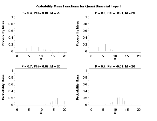
        
    plot generated by sample program

Program 2:
     
    let p = 0.7
    let phi = 0.01
    let m = 20
    let psave = p
    let phisave = phi
    let y = quasi binomial type I rand numb for i = 1 1 500
    .
    let y3 xlow xhigh = integer frequency table y
    class lower -0.5
    class width 1
    class upper 20.5
    let y2 x2 = binned y
    .
    relative hist y2 x2
    multiplot 2 2 4
    limits freeze
    pre-erase off
    line color blue
    plot qbipdf(x,p,phi,m) for x = 0 1 20
    limits
    pre-erase on
    line color black
    .
    quasi binomial type I mle y
    let p = pml
    let phi = phiml
    .
    quasi binomial type I chi-square goodness of fit y3 xlow xhigh
    .
    char x
    line bl
    quasi binomial type I probability plot y3 xlow xhigh
    .
    char bl
    line so
    let p1 = 0.5
    let p2 = 0.9
    let a1 = (1 - p1)/m
    let a2 = (1 - p2)/m
    let phi1 = 0
    let phi2 = max(a1,a2)
    quasi binomial type I ks plot y3 xlow xhigh
    let p = shape1
    let phi = shape2
    quasi binomial type I chi-square goodness of fit y3 xlow xhigh
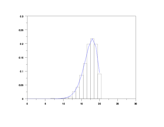
        
    plot generated by sample program
               QUASI BINOMIAL TYPE I PARAMETER ESTIMATION:
      
     NUMBER OF OBSERVATIONS                   =      500
     SAMPLE MEAN                              =    17.26600
     SAMPLE STANDARD DEVIATION                =    1.901177
     SAMPLE MINIMUM                           =    7.000000
     SAMPLE MAXIMUM                           =    20.00000
     ZERO-CLASS FREQUENCY:                    =    0.000000
      
     USER-SPECIFIED VALUE FOR M               =    20.00000
     MAXIMUM LIKELIHOOD:
     ESTIMATE OF P                            =   0.7056712
     ESTIMATE OF PHI                          =   0.9720844E-02
      
      
     THE COMPUTED VALUE OF THE CONSTANT P        =   0.7056712E+00
      
     THE COMPUTED VALUE OF THE CONSTANT PHI      =   0.9720844E-02
      
                       CHI-SQUARED GOODNESS-OF-FIT TEST
      
     NULL HYPOTHESIS H0:      DISTRIBUTION FITS THE DATA
     ALTERNATE HYPOTHESIS HA: DISTRIBUTION DOES NOT FIT THE DATA
     DISTRIBUTION:            QUASI BINOMIAL TYPE I
      
     SAMPLE:
        NUMBER OF OBSERVATIONS      =      500
        NUMBER OF NON-EMPTY CELLS   =        9
        NUMBER OF PARAMETERS USED   =        3
      
     TEST:
     CHI-SQUARED TEST STATISTIC     =    1.331433
        DEGREES OF FREEDOM          =        5
        CHI-SQUARED CDF VALUE       =    0.068336
      
        ALPHA LEVEL         CUTOFF              CONCLUSION
                10%        9.23636               ACCEPT H0
                 5%       11.07050               ACCEPT H0
                 1%       15.08628               ACCEPT H0
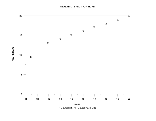
        
    plot generated by sample program

    plot generated by sample program

                       CHI-SQUARED GOODNESS-OF-FIT TEST
      
     NULL HYPOTHESIS H0:      DISTRIBUTION FITS THE DATA
     ALTERNATE HYPOTHESIS HA: DISTRIBUTION DOES NOT FIT THE DATA
     DISTRIBUTION:            QUASI BINOMIAL TYPE I
      
     SAMPLE:
        NUMBER OF OBSERVATIONS      =      500
        NUMBER OF NON-EMPTY CELLS   =        9
        NUMBER OF PARAMETERS USED   =        3
      
     TEST:
     CHI-SQUARED TEST STATISTIC     =    2.357771
        DEGREES OF FREEDOM          =        5
        CHI-SQUARED CDF VALUE       =    0.202254
      
        ALPHA LEVEL         CUTOFF              CONCLUSION
                10%        9.23636               ACCEPT H0
                 5%       11.07050               ACCEPT H0
                 1%       15.08628               ACCEPT H0
        

Date created: 8/23/2006
Last updated: 8/23/2006
Please email comments on this WWW page to alan.heckert@nist.gov.