TSSPDF
Name:
Type:
Purpose:
Compute the two-sided slope probability density function
with shape parameters
 and and
 . .
Description:
The standard two-sided slope distribution has the
following probability density function:
This distribution can be extended with lower and upper bound parameters.
If a and b denote the lower and upper bounds, respectively,
then the location and scale parameters are:
location = a
scale = b - a
The general form of the distribution can then be found
by using the relation
Syntax:
LET <y> = TSSPDF(<x>,<alpha>,<theta>,<a>,<b>)
<SUBSET/EXCEPT/FOR qualification>
where <x> is a number, parameter, or variable containing
values in the interval (a,b);
<y> is a variable or a parameter (depending on what
<x> is) where the computed two-sided slope pdf
value is stored;
<alpha> is a number, parameter, or variable in the
interval (0,2) that specifies the first shape
parameter;
<theta> is a number, parameter, or variable in the
interval (a,b) that specifies the second shape
parameter;
<a> is a number, parameter, or variable that
specifies the lower bound;
<b> is a number, parameter, or variable that
specifies the upper bound;
and where the <SUBSET/EXCEPT/FOR qualification> is optional.
If <a> and <b> are omitted, they default to 0 and 1,
respectively.
Examples:
LET A = TSSPDF(0.3,1.2,0.3)
LET Y = TSSPDF(X,1.5,2.2,0,5)
PLOT TSSPDF(X,1.5,2.2,0,5) FOR X = 0 0.01 5
Note:
Two-sided slope random numbers, probability plots, and
goodness of fit tests can be generated with the commands:
LET THETA = <value>
LET ALPHA = <value>
LET A = <value>
LET B = <value>
LET Y = TWO-SIDED SLOPE RANDOM NUMBERS FOR I = 1 1 N
TWO-SIDED SLOPE PROBABILITY PLOT Y
TWO-SIDED SLOPE PROBABILITY PLOT Y2 X2
TWO-SIDED SLOPE PROBABILITY PLOT Y3 XLOW XHIGH
TWO-SIDED SLOPE KOLMOGOROV SMIRNOV GOODNESS OF FIT Y
TWO-SIDED SLOPE CHI-SQUARE GOODNESS OF FIT Y2 X2
TWO-SIDED SLOPE CHI-SQUARE GOODNESS OF FIT Y3 XLOW XHIGH
Note that
A ≤ data minimum < THETA < data maximum ≤ B
The following commands can be used to estimate the
 and and
 shape parameters for the two-sided slope
distribution:
LET A = <value>
LET B = <value>
LET THETA1 = <value>
LET THETA2 = <value>
LET ALPHA1 = <value>
LET ALPHA2 = <value>
TWO-SIDED SLOPE PPCC PLOT Y
TWO-SIDED SLOPE PPCC PLOT Y2 X2
TWO-SIDED SLOPE PPCC PLOT Y3 XLOW XHIGH
TWO-SIDED SLOPE KS PLOT Y
TWO-SIDED SLOPE KS PLOT Y2 X2
TWO-SIDED SLOPE KS PLOT Y3 XLOW XHIGH
Note that for the two-sided slope distribution, the shape parameter
 is bounded by the minimum and maximum of the data. In the above commands,
there are two approaches to dealing with this.
- Specify the values for A and B (i.e., the
LET A = <value> and LET B = <value> commands).
The advantage of this approach is that
 is estimated in units of the data. The disadvantage
is that we lose the invariance of location and
scale for the PPCC plot (i.e., we cannot obtain
estimates of A and B).
- Use A = 0 and B = 1 (i.e., the standard form of
the distribution). This restricts the value of
 to the (0,1) interval.
The advantage of this approach is that we maintain
the invariance of location and scale for the
PPCC plot and can obtain indpendent estimates for
A and B.
The disadvantage of this approach is that we
have to scale the estimate of
 if the data are outside of the (0,1) interval.
To scale the estimate of
 in this method, do something like the following:
DELETE A B
LET YMIN = MINIMUM Y
LET YMAX = MAXIMUM Y
TWO-SIDED SLOPE PPCC PLOT Y
LET ALPHA = SHAPE1
LET THETA = SHAPE2
TWO SIDED SLOPE PROBABILITY PLOT Y
LET A = PPA0
LET B = A + PPA1
LET A = MIN(A,YMIM)
LET B = MAX(B,YMAX)
LET THETA = A + (B-A)*THETA
We include a check to make sure that the estimated
values for A and B are permissable (i.e., A ≤ YMIN
and B ≥ YMAX).
The default values for ALPHA1 and ALPHA2 are 0.05 and 2.
Default:
Synonyms:
Related Commands:
|
TSSCDF
|
= Compute the two-sided slope cumulative distribution function.
|
|
TSSPPF
|
= Compute the two-sided slope percent point function.
|
|
SLOPDF
|
= Compute the slope probability density function.
|
|
OGIPDF
|
= Compute the ogive probability density function.
|
|
TSOPDF
|
= Compute the two-sided ogive probability density function.
|
|
TOPPDF
|
= Compute the Topp and Leone probability density function.
|
|
RGTPDF
|
= Compute the generalized reflected Topp and Leone probability
density function.
|
|
GTLPDF
|
= Compute the generalized Topp and Leone probability density
function.
|
|
TSPPDF
|
= Compute the two-sided power probability density function.
|
|
BETPDF
|
= Compute the beta probability density function.
|
|
TRIPDF
|
= Compute the triangular probability density function.
|
|
TRAPDF
|
= Compute the trapezoid probability density function.
|
|
UNIPDF
|
= Compute the uniform probability density function.
|
|
POWPDF
|
= Compute the power probability density function.
|
|
JSBPDF
|
= Compute the Johnson SB probability density function.
|
Reference:
Samuel Kotz and J. Rene Van Dorp 2004, "Beyond Beta:
Other Continuous Families of Distributions with Bounded
Support and Applications", World Scientific, chapter 8.
Applications:
Implementation Date:
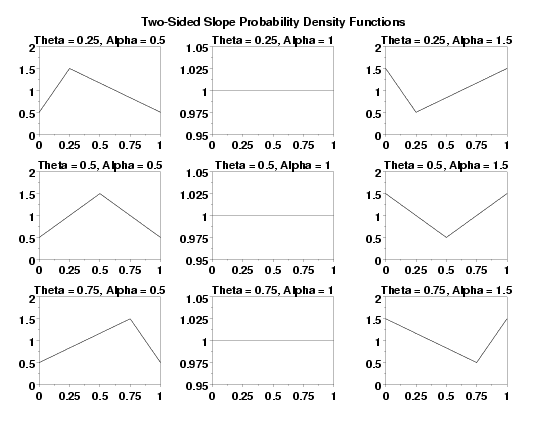
Program 1:
MULTIPLOT 3 3
MULTIPLOT CORNER COORDINATES 0 0 100 95
MULTIPLOT SCALE FACTOR 3
TITLE OFFSET 2
TITLE CASE ASIS
LABEL CASE ASIS
CASE ASIS
.
LET THETAV = DATA 0.25  0.50 0.75
LET ALPHAV = DATA 0.5  1.0  1.5
.
LOOP FOR K = 1 1 3
   LET THETA = THETAV(K)
   LOOP FOR L = 1 1 3
      LET ALPHA = ALPHAV(L)
      TITLE Theta = ^THETA, Alpha = ^ALPHA
      PLOT TSSPDF(X,ALPHA,THETA) FOR X = 0  0.01  1
   END OF LOOP
END OF LOOP
.
END OF MULTIPLOT
MOVE 50 97
JUSTIFICATION CENTER
TEXT Two-Sided Slope Probability Density Functions

Program 2:
let a = 0
let b = 4
let alpha = 1.3
let theta = 1.7
let alphasv = alpha
let thetasv = theta
.
let y = two-sided slope random numbers for i = 1 1 200
let ymin = minimum y
let ymax = maximum y
.
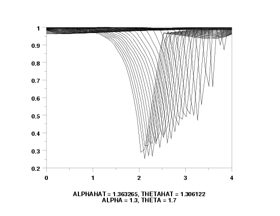
two-sided slope ppcc plot y
let alpha = shape1
let theta = shape2
justification center
move 50 6
text Alphahat = ^alpha, Thetahat = ^theta
move 50 3
text Alpha = ^alphasv, Theta = ^thetasv
.
char x
line bl
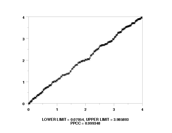
two-sided slope prob plot y
move 50 6
let ahat = ppa0
let bhat = ppa0 + ppa1
let ahat = min(ahat,ymin)
let bhat = max(bhat,ymax)
text Lower Limit = ^ppa0, Upper Limit = ^bhat
move 50 3
text PPCC = ^ppcc
.
two sided slope kolm smir goodness of fit y

                   KOLMOGOROV-SMIRNOV GOODNESS-OF-FIT TEST

 NULL HYPOTHESIS H0:      DISTRIBUTION FITS THE DATA
 ALTERNATE HYPOTHESIS HA: DISTRIBUTION DOES NOT FIT THE DATA
 DISTRIBUTION:            TWO-SIDED SLOPE
    NUMBER OF OBSERVATIONS              =      200

 TEST:
 KOLMOGOROV-SMIRNOV TEST STATISTIC      =   0.4090971E-01

    ALPHA LEVEL         CUTOFF              CONCLUSION
            10%       0.086*              ACCEPT H0
                      0.085**
             5%       0.096*              ACCEPT H0
                      0.095**
             1%       0.115*              ACCEPT H0
                      0.114**

     *  - STANDARD LARGE SAMPLE APPROXIMATION  ( C/SQRT(N) )
    ** - MORE ACCURATE LARGE SAMPLE APPROXIMATION  ( C/SQRT(N + SQRT(N/10)) )
Date created: 11/07/2007
Last updated: 11/07/2007
Please email comments on this WWW page to
alan.heckert@nist.gov.
|


 and
and
 .
.


