WAKPDF

WAKPDF (LET)

Library Function

Compute the Wakeby probability density function.

The Wakeby distribution is defined by the transformation

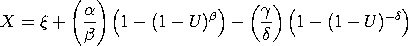
where U is a standard uniform random variable. That is, the above equation defines the percent point function for the Wakeby distribution.

The parameters , and are shape parameters. The parameter is a location parameter and the parameter is a location parameter.

The following restrictions apply to the parameters of this distribution:

1. + ≥ 0
2. Either + > 0 or = = = 0
3. If > 0, then > 0
4. ≥ 0
5. + ≥ 0

The domain of the Wakeby distribution is

1. to
   if ≥ 0 and > 0
2. to + (/ ) - (/ )
   if < 0 or = 0

With three shape parameters, the Wakeby distribution can model a wide variety of shapes.

The cumulative distribution function is computed by numerically inverting the percent point function given above. The probability density function is then found by using the following relation (given on page 46 of Johnson, Kotz, and Balakrishnan):

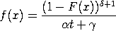
where F is the cumulative distribution function and

t = (1 - F(x)) ⁺

LET <y> = WAKPDF(<x>,<beta>,<gamma>,<delta>,<chi>,<alpha>)
                        <SUBSET/EXCEPT/FOR qualification>
where <x> is a number, parameter, or variable;
            <y> is a variable or a parameter (depending on what <x> is) where the computed Wakeby pdf value is stored;
            <beta> is a number, parameter, or variable that specifies the first shape parameter;
            <gamma> is a number, parameter, or variable that specifies the second shape parameter;
            <delta> is a number, parameter, or variable that specifies the third shape parameter;
            <chi> is a number, parameter, or variable that specifies the location parameter;
            <alpha> is a number, parameter, or variable that specifies the scale parameter;
and where the <SUBSET/EXCEPT/FOR qualification> is optional.

If <xi> and <alpha> are omitted, they default to 0 and 1, respectively.

LET A = WAKPDF(1.3,2.5,6)
LET A = WAKPDF(13,2.5,6,0,10)
PLOT WAKPDF(X,2.5,6) FOR X = -10 0.1 10

Wakeby uniform random numbers, probability plots, and goodness of fit tests can be generated with the commands:
LET BETA = <value>
LET GAMMA = <value>
LET DELTA = <value>
LET ALPHA = <value>
LET Y = WAKEBY RANDOM NUMBERS FOR I = 1 1 N
WAKEBY PROBABILITY PLOT Y
WAKEBY PROBABILITY PLOT Y2 X2
WAKEBY PROBABILITY PLOT Y3 XLOW XHIGH
WAKEBY KOLMOGOROV SMIRNOV GOODNESS OF FIT Y
WAKEBY CHI-SQUARE GOODNESS OF FIT Y2 X2
WAKEBY CHI-SQUARE GOODNESS OF FIT Y3 XLOW XHIGH


The parameters of the Wakeby distribution can be estimated by the method of L-moments using the command

WAKEBY MAXIMUM LIKELIHOOD Y

The cumulative distribution function for the Wakeby distribution is computed using the CDFWAK routine written by Hosking (see the Reference section below). Dataplot also uses Hoskings code for computing the L-moments parameter estimates.

Hoskings report and associated Fortran code can be downloaded from the Statlib archive at

http://lib.stat.cmu.edu/

None

None

WAKCDF	Compute the Wakeby cumulative distribution function.
WAKPPF	= Compute the Wakeby percent point function.
GEPPDF	= Compute the generalized Pareto probability density function.
GEVPDF	= Compute the generalized extreme value probability density function.
WEIPDF	= Compute the Weibull probability density function.
LGNPDF	= Compute the lognormal probability density function.
LAMPDF	Compute the Tukey lambda probability density function.
GLDPDF	= Compute the generalized Tukey lambda probability density function.
GHPDF	= Compute the g and h probability density function.

Johnson, Kotz, and Balakrishnan (1994), "Continuous Univariate Distribution--Volume 1", Second Edition, Wiley, pp. 44-47.

J. R. M. Hosking (2000), "Research Report: Fortran Routines for use with the Method of L-Moments", IBM Research Division, T. J. Watson Research Center, Yorktown Heights, NY 10598.

Hoskings (1990), "L-moments: Analysis and Estimation of Distribution using Linear Combinations of Order Statistics", Journal of the Royal Statistical Society, Series B, 52, pp. 105-124.

Distributional Modeling

2007/10

 
let xi = 0
let alpha = 10
let beta = 5
let gamma = 1
let delta = 0.3
.
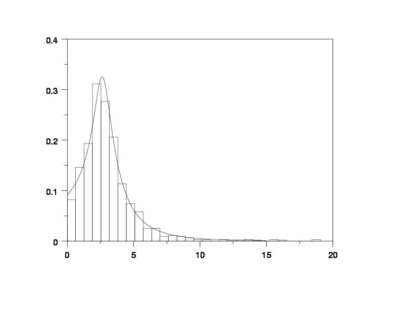
plot wakpdf(x,beta,gamma,delta,xi,alpha) for x = .01 .01 15
.
let y = wakeby rand numb for i = 1 1 1000
class lower 0
let a = maximum y
class upper a
relative hist y
limits freeze
pre-erase off
plot wakpdf(x,beta,gamma,delta,xi,alpha) for x = .01 .01 15
limits
pre-erase on
.
let xisv = xi
let alphasv = alpha
let betasv = beta
let gammasv = gamma
let deltasv = delta
.
wakeby mle y
let xi    = xilmom
let alpha = alphalmo
let beta  = betalmom
let gamma = gammalmo
let delta = deltalmo
.
wakeby kolmogorov smirnov goodness of fit y
.
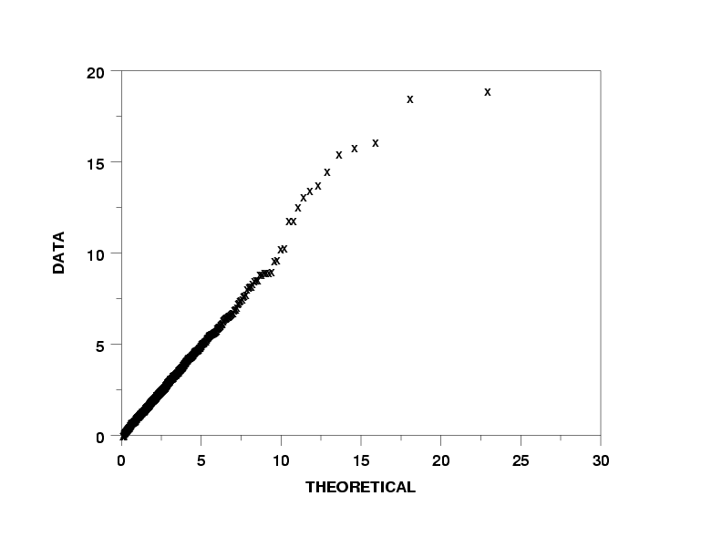
char x
line blank
y1label Data
x1label Theoretical
wakeby probability plot y
    



             WAKEBY PARAMETER ESTIMATION:
  
 SUMMARY STATISTICS:
 NUMBER OF OBSERVATIONS                     =     1000
 SAMPLE MEAN                                =    3.030319
 SAMPLE STANDARD DEVIATION                  =    2.118746
 SAMPLE MINIMUM                             =   0.3541647E-03
 SAMPLE MAXIMUM                             =    18.92599
  
 L-MOMENTS:
 FIRST SAMPLE L-MOMENT                      =    3.030319
 SECOND SAMPLE L-MOMENT                     =    1.016696
 THIRD SAMPLE L-MOMENT                      =   0.2496878
 THIRD SAMPLE L-MOMENT                      =   0.2474157
 THIRD SAMPLE L-MOMENT                      =   0.1351471
  
 ESTIMATE OF CHI                            =   0.5204416E-37
 ESTIMATE OF ALPHA                          =    9.342461
 ESTIMATE OF BETA                           =    5.207736
 ESTIMATE OF GAMMA                          =    1.090611
 ESTIMATE OF DELTA                          =   0.2351132
  
  
                   KOLMOGOROV-SMIRNOV GOODNESS-OF-FIT TEST
  
 NULL HYPOTHESIS H0:      DISTRIBUTION FITS THE DATA
 ALTERNATE HYPOTHESIS HA: DISTRIBUTION DOES NOT FIT THE DATA
 DISTRIBUTION:            WAKEBY
    NUMBER OF OBSERVATIONS              =     1000
  
 TEST:
 KOLMOGOROV-SMIRNOV TEST STATISTIC      =   0.1757836E-01
  
    ALPHA LEVEL         CUTOFF              CONCLUSION
            10%       0.039*              ACCEPT H0
                      0.038**
             5%       0.043*              ACCEPT H0
                      0.043**
             1%       0.052*              ACCEPT H0
                      0.051**
  
     *  - STANDARD LARGE SAMPLE APPROXIMATION  ( C/SQRT(N) )
    ** - MORE ACCURATE LARGE SAMPLE APPROXIMATION  ( C/SQRT(N + SQRT(N/10)) )