3. Production Process Characterization
3.5. Case Studies
3.5.1. Furnace Case Study

3.5.1.2.

Initial Analysis of Response Variable

Initial Plots of Response Variable

The initial step is to assess data quality and to look for anomalies. This is done by generating a normal probability plot, a histogram, and a boxplot. For convenience, these are generated on a single page.

Conclusions From the Plots

We can make the following conclusions based on these initial plots.

• The box plot indicates one outlier. However, this outlier is only slightly smaller than the other numbers.

• The normal probability plot and the histogram (with an overlaid normal density) indicate that this data set is reasonably approximated by a normal distribution.

Parameter Estimates

Parameter estimates for the film thickness are summarized in the following table. Parameter Estimates Type Parameter Estimate Lower (95%) Confidence Bound Upper (95%) Confidence Bound Location Mean 563.0357 559.1692 566.9023 Dispersion Standard Deviation 25.3847 22.9297 28.4331

Quantiles	Quantiles for the film thickness are summarized in the following table. Quantiles for Film Thickness 100.0% Maximum 634.00 99.5%   634.00 97.5%   615.10 90.0%   595.00 75.0% Upper Quartile 582.75 50.0% Median 562.50 25.0% Lower Quartile 546.25 10.0%   532.90 2.5%   514.23 0.5%   487.00 0.0% Minimum 487.00
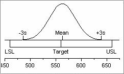
Capability Analysis	From the above preliminary analysis, it looks reasonable to proceed with the capability analysis. Dataplot generated the following capabilty analysis. **************************************************** * CAPABILITY ANALYSIS * * NUMBER OF OBSERVATIONS = 168 * * MEAN = 563.03571 * * STANDARD DEVIATION = 25.38468 * **************************************************** * LOWER SPEC LIMIT (LSL) = 460.00000 * * UPPER SPEC LIMIT (USL) = 660.00000 * * TARGET (TARGET) = 560.00000 * * USL COST (USLCOST) = UNDEFINED * **************************************************** * CP = 1.31313 * * CP LOWER 95% CI = 1.17234 * * CP UPPER 95% CI = 1.45372 * * CPL = 1.35299 * * CPL LOWER 95% CI = 1.21845 * * CPL UPPER 95% CI = 1.48753 * * CPU = 1.27327 * * CPU LOWER 95% CI = 1.14217 * * CPU UPPER 95% CI = 1.40436 * * CPK = 1.27327 * * CPK LOWER 95% CI = 1.12771 * * CPK UPPER 95% CI = 1.41882 * * CNPK = 1.35762 * * CPM = 1.30384 * * CPM LOWER 95% CI = 1.16405 * * CPM UPPER 95% CI = 1.44344 * * CC = 0.00460 * * ACTUAL % DEFECTIVE = 0.00000 * * THEORETICAL % DEFECTIVE = 0.00915 * * ACTUAL (BELOW) % DEFECTIVE = 0.00000 * * THEORETICAL(BELOW) % DEFECTIVE = 0.00247 * * ACTUAL (ABOVE) % DEFECTIVE = 0.00000 * * THEORETICAL(ABOVE) % DEFECTIVE = 0.00668 * * EXPECTED LOSS = UNDEFINED * ****************************************************
Summary of Percent Defective	From the above capability analysis output, we can summarize the percent defective (i.e., the number of items outside the specification limits) in the following table. Percentage Outside Specification Limits Specification Value Percent Actual Theoretical (% Based On Normal) Lower Specification Limit 460 Percent Below LSL = 100* ((LSL - )/s) 0.0000 0.0025% Upper Specification Limit 660 Percent Above USL = 100*(1 - ((USL - )/s)) 0.0000 0.0067% Specification Target 560 Combined Percent Below LSL and Above USL 0.0000 0.0091% Standard Deviation 25.38468       with denoting the normal cumulative distribution function, the sample mean, and s the sample standard deviation.
Summary of Capability Index Statistics	From the above capability analysis output, we can summarize various capability index statistics in the following table. Capability Index Statistics Capability Statistic Index Lower CI Upper CI CP 1.313 1.172 1.454 CPK 1.273 1.128 1.419 CPM 1.304 1.165 1.442 CPL 1.353 1.218 1.488 CPU 1.273 1.142 1.404
Conclusions	The above capability analysis indicates that the process is capable and we can proceed with the analysis.