Next Page Previous Page Home Tools & Aids Search Handbook
6. Process or Product Monitoring and Control
6.4. Introduction to Time Series Analysis
6.4.4. Univariate Time Series Models

6.4.4.10.

Box-Jenkins Analysis of Seasonal Data

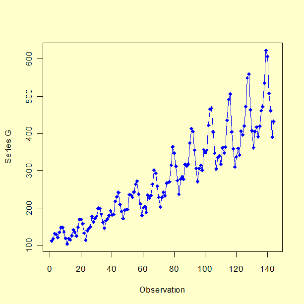
Series G This example illustrates a Box-Jenkins time series analysis for seasonal data using the series G data set in Box, Jenkins, and Reinsel, 1994. A plot of the 144 observations is shown below.
Plot of Series G Data
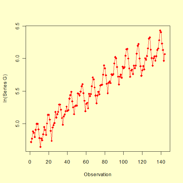
Non-constant variance can be removed by performing a natural log transformation.
Plot of natural log of series G
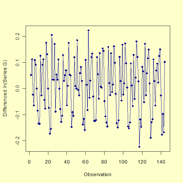
Next, we remove trend in the series by taking first differences. The resulting series is shown below.
Plot of first differences of the natural log of series G
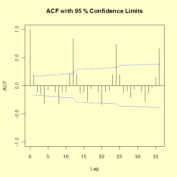
Analyzing Autocorrelation Plot for Seasonality To identify an appropriate model, we plot the ACF of the time series.
ACF plot of first differenced natural log series G
If very large autocorrelations are observed at lags spaced n periods apart, for example at lags 12 and 24, then there is evidence of periodicity. That effect should be removed, since the objective of the identification stage is to reduce the autocorrelation throughout. So if simple differencing is not enough, try seasonal differencing at a selected period, such as 4, 6, or 12. In our example, the seasonal period is 12.

A plot of Series G after taking the natural log, first differencing, and seasonal differencing is shown below.
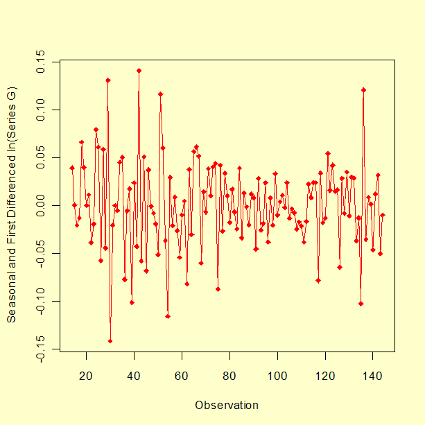
Seasonal and first differenced natural log of series G
The number of seasonal terms is rarely more than one. If you know the shape of your forecast function, or you wish to assign a particular shape to the forecast function, you can select the appropriate number of terms for seasonal AR or seasonal MA models.

The book by Box and Jenkins, Time Series Analysis Forecasting and Control (the later edition is Box, Jenkins and Reinsel, 1994) has a discussion on these forecast functions on pages 326 - 328. Again, if you have only a faint notion, but you do know that there was a trend upwards before differencing, pick a seasonal MA term and see what comes out in the diagnostics.

An ACF plot of the seasonal and first differenced natural log of series G is shown below.
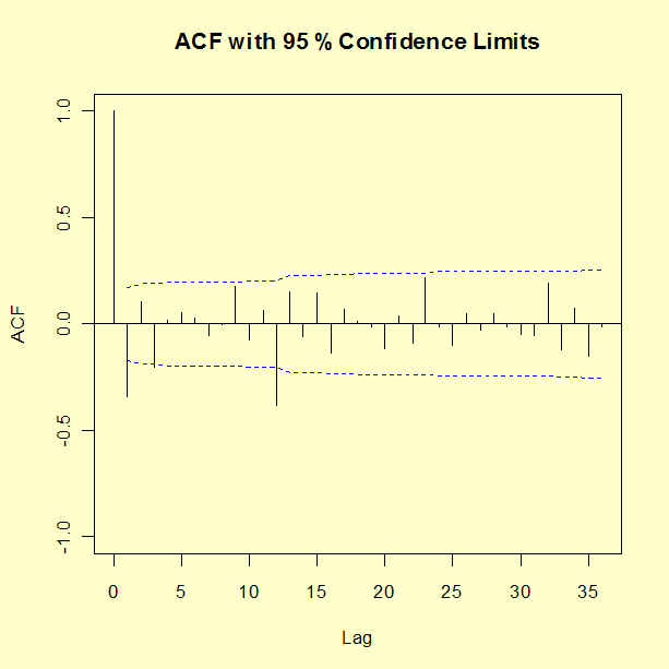
Autocorrelation plot after taking seasonal difference
The plot has a few spikes, but most autocorrelations are near zero, indicating that a seasonal MA(1) model is appropriate.
Model Fitting We fit a seasonal MA(1) model to the data $$ X_t - \delta = A_t + \theta_1 \, A_{t-1} + \psi_1 \, A_{t-12} + \theta_1 \, \psi_1 \, A_{t-13} \, , $$ where \(\theta_1\) represents the MA(1) parameter and \(\psi_1\) represents the seasonal parameter. The model fitting results are shown below.
                            Seasonal
Estimate            MA(1)     MA(1)
--------          -------    -------
Parameter         -0.4018    -0.5569
Standard Error     0.0896     0.0731

Residual standard deviation = 0.0367  
Log likelihood = 244.7
AIC = -483.4
Test the randomness of the residuals up to 30 lags using the Box-Ljung test. Recall that the degrees of freedom for the critical region must be adjusted to account for two estimated parameters.
H0:  The residuals are random.
Ha:  The residuals are not random.  

Test statistic:  Q = 29.4935
Significance level:  α = 0.05
Degrees of freedom:  h = 30 - 2 = 28
Critical value:  Χ 21-α,h = 41.3371 
Critical region: Reject H0 if Q > 41.3371
Since the null hypothesis of the Box-Ljung test is not rejected we conclude that the fitted model is adequate.
Forecasting Using our seasonal MA(1) model, we forcast values 12 periods into the future and compute 90 % confidence limits.
              Lower                   Upper
    Period    Limit      Forecast     Limit
    ------   --------    --------    --------
      145    424.0234    450.7261    478.4649
      146    396.7861    426.0042    456.7577
      147    442.5731    479.3298    518.4399
      148    451.3902    492.7365    537.1454
      149    463.3034    509.3982    559.3245
      150    527.3754    583.7383    645.2544
      151    601.9371    670.4625    745.7830
      152    595.7602    667.5274    746.9323
      153    495.7137    558.5657    628.5389
      154    439.1900    497.5430    562.8899
      155    377.7598    430.1618    489.1730
      156    417.3149    477.5643    545.7760
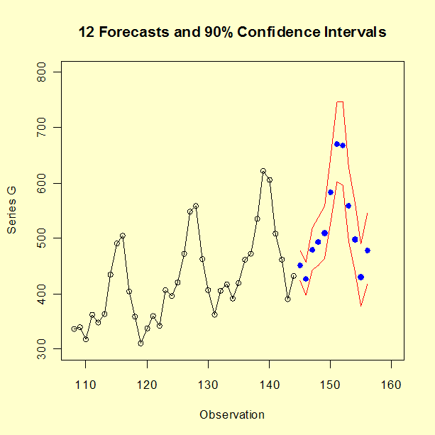
Plot of forecasted values with 90 % confidence limits
All the anlayses in this page can be generated using R code.
Home Tools & Aids Search Handbook Previous Page Next Page