DISTRIBUTIONAL FIT PLOT

DISTRIBUTIONAL FIT PLOT

Graphics Command

Generate a tabulation plot based on the results of the BEST DISTRIBUTIONAL FIT command.

The BEST DISTRIBUTIONAL FIT command generates a ranked list of best distributional fit for univariate data. This is a screening tool to identify good candidate distributional models for the data.

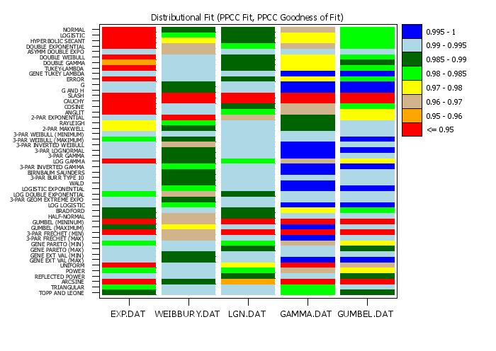
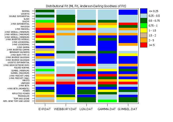
Often we have a number of related datasets. The DISTRIBUTIONAL FIT PLOT provides a convenient way of graphically presenting the results of the BEST DISTRIBUTIONAL FIT command for these multiple datasets. Specifically, it creates a tabulation plot where the y-axis contains the distribution and the x-axis contains the distinct datasets. That is, we can view a row of the plot to see how a particular distribution fits the various datasets and we can view a column to see which distributions fit a a particular dataset well.

There are two steps in the distributional modeling:

1. Fitting
2. Ranking by a goodness of fit critierion

You can specify the fit method with the command

SET BEST FIT METHOD <value>

where <value> is one of the following

MAXIMUM LIKELIHOOD:	maximum likelihood
PPCC:	PPCC goodness of fit
ANDERSON DARLING:	Anderson-Darling goodness of fit
KOLMOGOROV SMIRNOV:	Kolmogorov-Smirnov goodness of fit

The default method is maximum likelihood.

You can specify the goodness of fit critierion with the command

SET BEST FIT CRITERION <value>

where <value> is one of the following

ANDERSON DARLING:	Anderson-Darling
KOLMOGOROV SMIRNOV:	Kolmogorov-Smirnov
PPCC:	PPCC
AIC:	Akaike Information Criterion
AICc:	Akaike Information Criterion corrected for sample size
BIC:	Bayesian Information Criterion

The default goodness of fit criterion is Anderson-Darling.

Once the matrix (rows represent distribtions, columns represent datasets) of goodness of fit statistics is computed, they are plotted in the form of a tabulation plot. The tabulation plot is a mix between a fluctuation plot and a contour plot.

For the fluctuation plot, at each grid position, two rectangles are drawn. The first is drawn in a background color and is full size (i.e., the maximum value of the statistic). A second rectangle is drawn in a foreground color with a height proportional to the value of the statistic for that particular combination of categories.

For the tabulation plot, only one rectangle is drawn. However, the color of the rectangle is based on the value of the statistic relative to a "levels" variable (hence the similarity to a contour plot). The Program examples below demonstrate how to create and use the levels variable. Note that defining good levels for the information criterion goodness of fit statistics is somewhat problematic, so this plot is more useful for the PPCC, Anderson-Darling, and Kolmogorov-Smirnov goodness of fit statistics.

The appearance of the tabulation plot is controlled by appropriate settings for the REGION, LINE, and CHARACTER settings. This is demonstrated in the Program examples below.

Note that not all of the options available for a standard TABULATION PLOT are supported for this command.

DISTRIBUTIONAL FIT PLOT <y> <x> <ylevel>
                        <SUBSET/EXCEPT/FOR qualification>
where <y> is a response variable;
            <x> is a group-id variable;
            <ylevel> is a variable that defines the levels;
and where the <SUBSET/EXCEPT/FOR qualification> is optional.

For this syntax, the different datasets are identified by a group-id variable.

MULTIPLE DISTRIBUTIONAL FIT PLOT <y1> ... <yk> <ylevel>
                        <SUBSET/EXCEPT/FOR qualification>
where <y1> ... <yk> is a list of 1 to 30 response variables;
            <ylevel> is a variable that defines the levels;
and where the <SUBSET/EXCEPT/FOR qualification> is optional.

For this syntax, the different datasets are identified with separate response variables.

REPLICATED DISTRIBUTIONAL FIT PLOT <y> <x1> ... <xk> <ylevel>
                        <SUBSET/EXCEPT/FOR qualification>
where <y> is a response variable;
            <x1> ... <x6> is a list of 1 to 6 group-id variables;
            <ylevel> is a variable that defines the levels;
and where the <SUBSET/EXCEPT/FOR qualification> is optional.

The group-id variables are cross-tabulated and a dataset is defined for each distinct combination of values for the group-id variables.

For the REPLICATED case, you can control the spacing between groups. Internally, Dataplot uses the CODE CROSS TABULATE command to generate a single combined group-id variable. Enter HELP CODE CROSS TABULATE for details on how to control the spacing (the SET commands used by CODE CROSS TABULATE are supported for the DISTRIBUTIONAL FIT PLOT command).

DISTRIBUTIONAL FIT PLOT Y X
MULTIPLE DISTRIBUTIONAL FIT PLOT Y1 TO Y8
REPLICATED DISTRIBUTIONAL FIT PLOT Y X1 X2
DISTRIBUTIONAL FIT PLOT Y X SUBSET X < 8

The following command was added
SET TABULATION PLOT CODED <ON/OFF>

By default (= ON), each factor variable is coded from 1 to NDIST with NDIST denoting the number of levels (i.e., distinct values for that factor variable).

When this switch is set to OFF, the x-axis variable is plotted in the units of group-id variable. This can be useful if you want to add spacing between some groups of data or if you have missing groups that you want the plot to clearly show.

This command does not apply for Syntax 2 (the MULTIPLTE option).

The 2020/05 version of Dataplot added the ability to specify which distributions to include. The following commands were added
SET BEST FIT DISTRIBUTION NORMAL <ON/OFF>
SET BEST FIT DISTRIBUTION LOGISTIC <ON/OFF>
SET BEST FIT DISTRIBUTION LOG LOGISTIC <ON/OFF>
SET BEST FIT DISTRIBUTION HYPERBOLIC SECANT <ON/OFF>
SET BEST FIT DISTRIBUTION UNIFORM <ON/OFF>
SET BEST FIT DISTRIBUTION POWER <ON/OFF>
SET BEST FIT DISTRIBUTION ARCSINE <ON/OFF>
SET BEST FIT DISTRIBUTION TRIANGULAR <ON/OFF>
SET BEST FIT DISTRIBUTION ERROR <ON/OFF>
SET BEST FIT DISTRIBUTION SLASH <ON/OFF>
SET BEST FIT DISTRIBUTION CAUCHY <ON/OFF>
SET BEST FIT DISTRIBUTION COSINE <ON/OFF>
SET BEST FIT DISTRIBUTION BRADFORD <ON/OFF>
SET BEST FIT DISTRIBUTION ANGLIT <ON/OFF>
SET BEST FIT DISTRIBUTION RAYLEIGH <ON/OFF>
SET BEST FIT DISTRIBUTION FOLDED NORMAL <ON/OFF>
SET BEST FIT DISTRIBUTION TUKEY LAMBDA <ON/OFF>
SET BEST FIT DISTRIBUTION GENERALIZED TUKEY LAMBDA <ON/OFF>
SET BEST FIT DISTRIBUTION DOUBLE GAMMA <ON/OFF>
SET BEST FIT DISTRIBUTION DOUBLE WEIBULL <ON/OFF>
SET BEST FIT DISTRIBUTION REFLECTED POWER <ON/OFF>
SET BEST FIT DISTRIBUTION TWO SIDED POWER <ON/OFF>
SET BEST FIT DISTRIBUTION TOPP AND LEONE <ON/OFF>
SET BEST FIT DISTRIBUTION REFLECTED GENERALIZED TOPP AND LEONE <ON/OFF>
SET BEST FIT DISTRIBUTION GENERALIZED EXTREME VALUE MINIMUM <ON/OFF>
SET BEST FIT DISTRIBUTION GENERALIZED EXTREME VALUE MAXIMUM <ON/OFF>
SET BEST FIT DISTRIBUTION PARETO <ON/OFF>
SET BEST FIT DISTRIBUTION GENERALIZED PARETO MINIMUM <ON/OFF>
SET BEST FIT DISTRIBUTION GENERALIZED PARETO MAXIMUM <ON/OFF>
SET BEST FIT DISTRIBUTION G AND H <ON/OFF>
SET BEST FIT DISTRIBUTION G <ON/OFF>
SET BEST FIT DISTRIBUTION INVERTED WEIBULL <ON/OFF>
SET BEST FIT DISTRIBUTION GAMMA <ON/OFF>
SET BEST FIT DISTRIBUTION LOG GAMMA <ON/OFF>
SET BEST FIT DISTRIBUTION INVERTED GAMMA <ON/OFF>
SET BEST FIT DISTRIBUTION FATIGUE LIFE <ON/OFF>
SET BEST FIT DISTRIBUTION WALD <ON/OFF>
SET BEST FIT DISTRIBUTION LOGISTIC EXPONENTIAL <ON/OFF>
SET BEST FIT DISTRIBUTION GEOMETRIC EXTREME EXPONENTIAL <ON/OFF>
SET BEST FIT DISTRIBUTION LOG DOUBLE EXPONENTIAL <ON/OFF>


SET BEST FIT DISTRIBUTION TWO PARAMETER LOGNORMAL <ON/OFF>
SET BEST FIT DISTRIBUTION 2 PARAMETER LOGNORMAL <ON/OFF>


SET BEST FIT DISTRIBUTION THREE PARAMETER LOGNORMAL <ON/OFF>
SET BEST FIT DISTRIBUTION 3 PARAMETER LOGNORMAL <ON/OFF>


SET BEST FIT DISTRIBUTION TWO PARAMETER EXPONENTIAL <ON/OFF>
SET BEST FIT DISTRIBUTION 2 PARAMETER EXPONENTIAL <ON/OFF>
SET BEST FIT DISTRIBUTION EXPONENTIAL <ON/OFF>


SET> BEST FIT DISTRIBUTION TWO PARAMETER WEIBULL MINIMUM <ON/OFF>
SET> BEST FIT DISTRIBUTION 2 PARAMETER WEIBULL MINIMUM <ON/OFF>
SET> BEST FIT DISTRIBUTION TWO PARAMETER WEIBULL <ON/OFF>
SET> BEST FIT DISTRIBUTION 2 PARAMETER WEIBULL <ON/OFF>


SET BEST FIT DISTRIBUTION TWO PARAMETER WEIBULL MAXIMUM <ON/OFF>
SET BEST FIT DISTRIBUTION 2 PARAMETER WEIBULL MAXIMUM <ON/OFF>


SET BEST FIT DISTRIBUTION THREE PARAMETER WEIBULL MINIMUM <ON/OFF>
SET BEST FIT DISTRIBUTION 3 PARAMETER WEIBULL MINIMUM <ON/OFF>
SET BEST FIT DISTRIBUTION THREE PARAMETER WEIBULL <ON/OFF>
SET BEST FIT DISTRIBUTION 3 PARAMETER WEIBULL <ON/OFF>


SET BEST FIT DISTRIBUTION THREE PARAMETER WEIBULL MAXIMUM <ON/OFF>
SET BEST FIT DISTRIBUTION 3 PARAMETER WEIBULL MAXIMUM <ON/OFF>


SET BEST FIT DISTRIBUTION <E PARAMETER EXPONENTIAL ON/OFF>
SET BEST FIT DISTRIBUTION 1 PARAMETER EXPONENTIAL <ON/OFF>


SET BEST FIT DISTRIBUTION ASYMMETRIC DOUBLE EXPONENTIAL <ON/OFF>
SET BEST FIT DISTRIBUTION ASYMMETRIC LAPLACE <ON/OFF>


SET> BEST FIT DISTRIBUTION DOUBLE EXPONENTIAL <ON/OFF>
SET> BEST FIT DISTRIBUTION LAPLACE <ON/OFF>


SET BEST FIT DISTRIBUTION BURR TYPE TEN <ON/OFF>
SET BEST FIT DISTRIBUTION BURR TYPE 10 <ON/OFF>


SET BEST FIT DISTRIBUTION TWO PARAMETER INVERSE GAUSSIAN <ON/OFF>
SET BEST FIT DISTRIBUTION 2 PARAMETER INVERSE GAUSSIAN <ON/OFF≶


SET BEST FIT DISTRIBUTION THREE PARAMETER INVERSE GAUSSIAN <ON/OFF>
SET BEST FIT DISTRIBUTION 3 PARAMETER INVERSE GAUSSIAN <ON/OFF>


SET BEST FIT DISTRIBUTION THREE PARAMETER LOGNORMAL <ON/OFF>
SET BEST FIT DISTRIBUTION 3 PARAMETER LOGNORMAL <ON/OFF>


SET BEST FIT DISTRIBUTION TWO PARAMETER EXPONENTIAL <ON/OFF>
SET BEST FIT DISTRIBUTION GUMBEL MINIMUM <ON/OFF>
SET BEST FIT DISTRIBUTION GUMBEL MAXIMUM <ON/OFF>
SET BEST FIT DISTRIBUTION EXTREME VALUE TYPE 1 MINIMUM <ON/OFF>
SET BEST FIT DISTRIBUTION EXTREME VALUE TYPE 1 MAXIMUM <ON/OFF>
SET BEST FIT DISTRIBUTION EXTREME VALUE TYPE I MINIMUM <ON/OFF>
SET BEST FIT DISTRIBUTION EXTREME VALUE TYPE I MAXIMUM <ON/OFF>


SET BEST FIT DISTRIBUTION FRECHET MINIMUM <ON/OFF>
SET BEST FIT DISTRIBUTION FRECHET MAXIMUM <ON/OFF>
SET BEST FIT DISTRIBUTION EXTREME VALUE TYPE TWO MINIMUM <ON/OFF>
SET BEST FIT DISTRIBUTION EXTREME VALUE TYPE TWO MAXIMUM <ON/OFF>
SET BEST FIT DISTRIBUTION EXTREME VALUE TYPE II MINIMUM <ON/OFF>
SET BEST FIT DISTRIBUTION EXTREME VALUE TYPE II MAXIMUM <ON/OFF>
SET BEST FIT DISTRIBUTION EXTREME VALUE TYPE 2 MINIMUM <ON/OFF>
SET BEST FIT DISTRIBUTION EXTREME VALUE TYPE 2 MAXIMUM <ON/OFF>


SET BEST FIT DISTRIBUTION TWO PARAMETER BETA <ON/OFF>
SET BEST FIT DISTRIBUTION 2 PARAMETER BETA <ON/OFF>


SET BEST FIT DISTRIBUTION FOUR PARAMETER BETA <ON/OFF>
SET BEST FIT DISTRIBUTION 4 PARAMETER BETA <ON/OFF>


SET BEST FIT DISTRIBUTION <E PARAMETER HALF NORMAL ON/OFF>
SET BEST FIT DISTRIBUTION 1 PARAMETER HALF NORMAL <ON/OFF>


SET BEST FIT DISTRIBUTION TWO PARAMETER HALF NORMAL <ON/OFF>
SET BEST FIT DISTRIBUTION 2 PARAMETER HALF NORMAL <ON/OFF>
SET BEST FIT DISTRIBUTION HALF NORMAL <ON/OFF>


SET BEST FIT DISTRIBUTION <E PARAMETER HALF LOGISTIC ON/OFF>
SET BEST FIT DISTRIBUTION 1 PARAMETER HALF LOGISTIC <ON/OFF>


SET BEST FIT DISTRIBUTION TWO PARAMETER HALF LOGISTIC <ON/OFF>
SET BEST FIT DISTRIBUTION 2 PARAMETER HALF LOGISTIC <ON/OFF>
SET BEST FIT DISTRIBUTION HALF LOGISTIC <ON/OFF>


SET BEST FIT DISTRIBUTION TWO COMPONENT NORMAL MIXTURE <ON/OFF>
SET BEST FIT DISTRIBUTION 2 COMPONENT NORMAL MIXTURE <ON/OFF>


The following resets the default list of distributions

SET BEST FIT DISTRIBUTION ALL
SET BEST FIT DISTRIBUTION DEFAULT


The following turns off all the distributions. If you have a small set of distributions, you can enter one of these commands first and then use the above commands to turn on the specific distributions you want to include

SET BEST FIT DISTRIBUTION NONE
SET BEST FIT DISTRIBUTION OFF

None

None

BEST DISTRIBUTIONAL FIT	= Generate a ranked list of best distributional fit.
GOODNESS OF FIT	= Perform a distributional goodness of fit.
TABULATION PLOT	= Generate a tabulation plot.
FLUCTUATION PLOT	= Generate a fluctuation plot.
CONTOUR PLOT	= Generate a contour plot.

Distributional Modeling

2014/09
2020/05: Added support for specifying which distribution to include

 
.
. Step 1:   Read the data
.
skip 25
read exp.dat       y1
read weibbury.dat  y2
read lgn.dat       y3
read gamma.dat     y4
read gumbel.dat    y5
skip 0
.
let string dist1 = EXP.DAT
let string dist2 = WEIBBURY.DAT
let string dist3 = LGN.DAT
let string dist4 = GAMMA.DAT
let string dist5 = GUMBEL.DAT
.
. Step 2:   Set basic plot control features
.
case asis
title case asis
label case asis
tic mark label case asis
title offset 1
title size 1.8
xlimits 1 5
major xtic mark number 5
minor xtic mark number 0
x1tic mark offset 0.5 0.5
x1tic mark label format alpha
x1tic mark label content  ^dist1 ^dist2 ^dist3 ^dist4 ^dist5
y1tic mark offset 1 1
y1tic mark label size 1.3
frame corner coordinates 15 15 80 93
.
. Step 3:   Define the plot levels
.
let p1 = 0.95
let p2 = 0.96
let p3 = 0.97
let p4 = 0.98
let p5 = 0.985
let p6 = 0.990
let p7 = 0.995
let p8 = 1.0001
let ylevel = data p1 p2 p3 p4 p5 p6 p7 p8
.
let ncolor = 8
let string color1 = red
let string color2 = orange
let string color3 = tan
let string color4 = yellow
let string color5 = green
let string color6 = dgreen
let string color7 = lblue
let string color8 = blue
.
. Step 4:   Define options and generate the plot
.
region fill on all
region fill color   ^color1 ^color2 ^color3 ^color4 ^color5 ^color6 ...
                    ^color7 ^color8
line color          white all
.
set write decimals 5
set best fit method     ppcc
set best fit criterion  ppcc
.
title Distributional Fit (PPCC Fit, PPCC Goodness of Fit)
multiple distributional fit  plot y1 to y5 ylevel
.
. Step 5:   Draw the legend box
.
box fill pattern solid
box shadow hw 0 0
justification left
height 1.7
.
let xcoor1 = 81
let xcoor2 = 85
let xcoor3 = xcoor2 + 1
let ycoor1 = 93
let yinc   = 4
let ycoor2 = ycoor1 - yinc
let kind = ncolor
.
loop for k = 1 1 ncolor
    box fill color ^color^kind
    box xcoor1 ycoor1 xcoor2 ycoor2
    let ycoor3 = ycoor2 + 1
    move xcoor3 ycoor3
    let km1 = kind - 1
    let aval1 = ^p^km1
    let aval2 = ^p^kind
    let aval2 = min(1,aval2)
    if k < ncolor
       if k = 1
          text ^aval1 - ^aval2
       else
          text ^aval1 - ^aval2
      end of if
    else
      text <= ^aval1
    end of if
    let ycoor1 = ycoor2
    let ycoor2 = ycoor1 - yinc
    let kind = kind - 1
end of loop
    

 
.
. Step 1:   Read the data
.
skip 25
read exp.dat       y1
read weibbury.dat  y2
read lgn.dat       y3
read gamma.dat     y4
read gumbel.dat    y5
skip 0
.
let string dist1 = EXP.DAT
let string dist2 = WEIBBURY.DAT
let string dist3 = LGN.DAT
let string dist4 = GAMMA.DAT
let string dist5 = GUMBEL.DAT
.
. Step 2:   Set basic plot control features
.
case asis
title case asis
label case asis
tic mark label case asis
title offset 1
title size 1.8
xlimits 1 5
major xtic mark number 5
minor xtic mark number 0
x1tic mark offset 0.5 0.5
x1tic mark label format alpha
x1tic mark label content  ^dist1 ^dist2 ^dist3 ^dist4 ^dist5
y1tic mark offset 1 1
y1tic mark label size 1.3
frame corner coordinates 15 15 80 93
y1tic mark offset 1 1
y1tic mark label size 1.3
.
. Step 3:   Define the plot levels
.
let p1 = 0.25
let p2 = 0.50
let p3 = 0.75
let p4 = 1.0
let p5 = 1.5
let p6 = 2.0
let p7 = 5.0
let p8 = 10000
let ylevel = data p1 p2 p3 p4 p5 p6 p7 p8
.
let ncolor = 8
let string color1 = blue
let string color2 = lblue
let string color3 = dgreen
let string color4 = green
let string color5 = yellow
let string color6 = tan
let string color7 = orange
let string color8 = red
.
. Step 4:   Define plot options and generate the plot
.
set write decimals 5
set best fit method     ml
set best fit criterion  anderson darling
.
region fill on all
region fill color   ^color1 ^color2 ^color3 ^color4 ^color5 ^color6 ...
                    ^color7 ^color8
line color          white all
.
title Distributional Fit (ML Fit, Anderson-Darling Goodness of Fit)
multiple distributional fit  plot y1 to y5  ylevel
.
. Step 5:   Add some labels and draw the legend box
.
box fill pattern solid
box shadow hw 0 0
justification left
height 1.7
.
let xcoor1 = 81
let xcoor2 = 85
let xcoor3 = xcoor2 + 1
let ycoor1 = 93
let yinc   = 4
let ycoor2 = ycoor1 - yinc
.
loop for k = 1 1 ncolor
    box fill color ^color^k
    box xcoor1 ycoor1 xcoor2 ycoor2
    let ycoor3 = ycoor2 + 1
    move xcoor3 ycoor3
    if k = 1
       text <= ^p1
    else if k = ncolor
       let km1 = k - 1
       text >= ^p^km1
    else
       let km1 = k - 1
       text ^p^km1 - ^p^k
    end of if
    let ycoor1 = ycoor2
    let ycoor2 = ycoor1 - yinc
end of loop