HISTOGRAM

... HISTOGRAM

Graphics Command

Generates a histogram.

A histogram is a graphical data analysis technique for summarizing the distributional information of a variable. The response variable is divided into equal sized intervals (or bins). The number of occurrences of the response variable is calculated for each bin. The histogram consists of:

Vertical axis	=	frequencies or relative frequencies;
Horizontal axis	=	response variable (i.e., the mid-point of each interval).

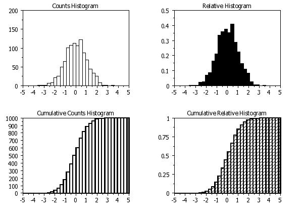
There are 4 types of histograms:

1. histogram (absolute counts);
2. relative histogram (converts counts to proportions);
3. cumulative histogram;
4. cumulative relative histogram.

The histogram and the frequency plot have the same information except the histogram has bars at the frequency values, whereas the frequency plot has lines connecting the frequency values.

<type> <x>             <SUBSET/EXCEPT/FOR qualification>
where <type> is one of HISTOGRAM, RELATIVE HISTOGRAM, CUMULATIVE HISTOGRAM, or CUMULATIVE RELATIVE HISTOGRAM;
            <x> is a variable of raw data values;
and where the <SUBSET/EXCEPT/FOR qualification is optional.

This syntax is used when you have raw data. Note that <x> can be either a variable or a matrix. If <x> is a matrix, then a histogram will be generated for all values in that matrix.

<type> <y> <x>             <SUBSET/EXCEPT/FOR qualification>
where <type> is one of HISTOGRAM, RELATIVE HISTOGRAM, CUMULATIVE HISTOGRAM, or CUMULATIVE RELATIVE HISTOGRAM;
            <y> is a variable containing pre-computed frequencies;
            <x> is a variable containing the bin mid-points;
and where the <SUBSET/EXCEPT/FOR qualification is optional.

This syntax is used when you have grouped data with equi-sized bins.

<type> <y> <xlow> <xhigh>             <SUBSET/EXCEPT/FOR qualification>
where <type> is one of HISTOGRAM, RELATIVE HISTOGRAM,
CUMULATIVE HISTOGRAM, or CUMULATIVE RELATIVE HISTOGRAM;
<y> is a variable containing pre-computed frequencies;
            <xlow> is a variable containing the lower limits for the bins;
            <xhigh> is a variable containing the upper limits for the bins; and where the <SUBSET/EXCEPT/FOR qualification is optional.

This syntax is used when you have grouped data with unequal sized bins.

SUBSET <type> <y> <x>             <SUBSET/EXCEPT/FOR qualification>
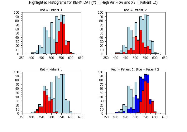
where <type> is one of HISTOGRAM, RELATIVE HISTOGRAM, CUMULATIVE HISTOGRAM, or CUMULATIVE RELATIVE HISTOGRAM;
            <y> is a variable of raw data values;
            <x> is a group-id variable; and where the <SUBSET/EXCEPT/FOR qualification is optional.

This syntax can be used to highlight the contribution to the histogram for particular subsets of the data. It is demonstrated in the program examples below.

HISTOGRAM TEMP
RELATIVE HISTOGRAM TEMP
CUMULATIVE HISTOGRAM TEMP
CUMULATIVE RELATIVE HISTOGRAM TEMP
HISTOGRAM COUNTS STATE
RELATIVE HISTOGRAM COUNTS STATE
CUMULATIVE HISTOGRAM COUNTS STATE
CUMULATIVE RELATIVE HISTOGRAM COUNTS STATE

There are two methods for relative histograms.

The first method simply divides the count in the bin by the total count. That is, the relative frequency of the i-th bin is \( n_{i}/\sum{n_{i}} \) where \( n_{i} \) is the count of the i-th bin. In this case, the sum of the relative frequencies is one. To specify this method, enter the command

SET RELATIVE HISTOGRAM PERCENT

The second method normalizes the counts so that the area sums to one. That is, the relative frequency of the i-th bin is \( n_{i}/\sum{n_{i} c_{i}} \) where \( c_{i} \) is the width of the i-th bin. To specify this method, enter the command

SET RELATIVE HISTOGRAM AREA

The advantage of the AREA method is that it makes the relative histogram an estimator of the underlying probability distribution. The histogram in this case is actually a simple kernel density estimator of the underlying distribution of the data. This is not the case when the PERCENT option is used.

The default is AREA.

The appearance of the bars on the histogram (i.e., whether they are filled or not, the line width of the bar border, etc.) are controlled by the various bar attribute commands. A few are listed in the RELATED COMMANDS section below. See the documentation for the BAR command for a complete list of the bar attribute commands. This is demonstrated with the sample program below.

You can extract a frequency table from the histogram with the following commands:
HISTOGRAM Y
LET YFREQ = YPLOT
LET XVAL = XPLOT


Then the variables YFREQ and XVAL contain a frequency table. You can also use the

LET Y2 X2 = BINNED Y

command for this purpose.

By default, DATAPLOT uses a class width of 0.3 X the standard deviation of the variable. Use the CLASS WIDTH command to override this default. DATAPLOT also tends to generate a large number of zero frequency classes at the lower and upper tails. This tends to compress the histogram on the horizontal axis. Use the XLIMITS command or the CLASS LOWER and CLASS UPPER commands to avoid plotting these zero frequency classes.

A number of alternative choices for class width can be set with the command

SET HISTOGRAM CLASS WIDTH

Enter HELP HISTOGRAM CLASS WIDTH for details.

By default, Dataplot sets the lower and upper class limits to xbar -/+ 6*s (with xbar and s denoting the sample mean and standard deviation, respectively). This can occassionally result in a few outlying points being excluded from the histogram. To adjust the lower and upper class limits so that these outlying points are included, enter the command
SET HISTOGRAM OUTLIERS ON

To revert to the default, enter

SET HISTOGRAM OUTLIERS OFF

By default, the histogram draws all cells, even those with zero frequency. To suppress these zero frequency cells, enter
SET HISTOGRAM EMPTY BINS OFF

To restore the default, enter

SET HISTOGRAM EMPTY BINS ON

Previously, Dataplot only generated histograms for the case where the bin widths were equal. This has been extended to the case with unequal bin widths. The syntax is
HISTOGRAM Y XLOW XHIGH

with XLOW containing the values for the lower bin limit and XHIGH containing the values for the upper bin limit.

Added the following option
SUBSET HISTOGRAM Y X

In this case, X is a group-id variable. This syntax can be used to highlight the contribution to the histogram for particular subsets of the data.

When dealing with pathological data sets (e.g., Cauchy distributed data), there is an issue with generating a class size that is appropriate for central bulk of the data while still being able to generate the histogram in an efficient fashion. The following commands provide some methods for addressing this.

When you have data where there are a small percentage of points that are quite far from the bulk of the data, you might want to use the command (this already existed, enter HELP HISTOGRAM CLASS WIDTH for details).

SET HISTOGRAM CLASS WIDTH IQ RANGE

This bases the bin width for the histogram on the interquartile range rather than the standard deviation as the other class width algorithms do. This can result in more reasonable class widths for the center of the data when there are extreme outliers in the data. Also, these commands are typically used when the

SET HISTOGRAM OUTLIERS ON

command is also given (this command extends the bins to cover all outliers).

1. The following command can be used to specify the maximum number of classes for the histogram.
   SET HISTOGRAM MAXIMUM CLASSES <value>

   If this command is entered, then the class width is initially computed in the standard way. If the number of bins needed to cover the outliers is greater than the value given here, then the class width is recomputed so that the number of bins is equal to the value given here.

2. The following command can be used to specify that outliers be drawn as individual points rather than extending the bins to cover them.
   SET HISTOGRAM OUTLIER POINTS ON

   To turn this option off, enter

   SET HISTOGRAM OUTLIER POINTS OFF

None

A synonym for CUMULATIVE RELATIVE HISTOGRAM is RELATIVE CUMULATIVE HISTOGRAM. HIGHLIGHT is a synonym for SUBSET in syntax 4.

FREQUENCY PLOT	= Generate a frequency plot.
KERNEL DENSITY PLOT	= Generate a kernel density plot.
PERCENT POINT PLOT	= Generate a percent point plot.
PROBABILITY PLOT	= Generate a probability plot.
PPCC PLOT	= Generates probability plot correlation coefficient plot.
PLOT	= Generate a data or function plot.
CLASS LOWER	= Set the lower class minimum for histograms, frequency plots, and pie charts.
CLASS UPPER	= Set the upper class maximum for histograms, frequency plots, and pie charts.
CLASS WIDTH	= Set the class width for histograms, frequency plots, and pie charts.
HISTOGRAM CLASS WIDTH	= Specify alternative default class wdith algorithms for histograms.
MINIMUM	= Set the frame minima for all plots.
MAXIMUM	= Set the frame maxima for all plots.
LIMITS	= Set the frame limits for all plots.
BARS	= Set the on/off switches for plot bars.
BAR WIDTH	= Set the widths for plot bars.
BAR FILL	= Set the on/off switches for plot bar fills.
BAR PATTERN	= Set the types for bar fill patterns.
BAR BORDER LINE	= Set the types for bar border lines.

NIST/SEMATECH e-Handbook of Statistical Methods, http://www.itl.nist.gov/div898/handbook/eda/section3/histogra.htm, 6/2003.

David Scott (1992), "Multivariate Density Estimation", John Wiley, (chapter 3). This book discusses histograms as "density estimators" and gives optimal criterion for selecting the class width.

Data Analysis

Pre-1987
2004/09: Support alternative class width algorithms
2007/03: Option to compute histogram of a matrix
2010/01: Support for HIGHLIGHT/SUBSET option
2010/01: Support for non-equispaced histograms
2010/01: Option to suppress empty bins
2010/01: Option to include outliers
2016/06: Support for SET HISTOGRAM MAXIMUM CLASSES
2016/06: Support for SET HISTOGRAM OUTLIER POINTS

 
LET Y = NORMAL RANDOM NUMBERS FOR I = 1 1 1000
MULTIPLOT 2 2
MULTIPLOT SCALE FACTOR 2
MULTIPLOT CORNER COORDINATES 0 0 100 100
XLIMITS -5 5
TITLE CASE ASIS
TITLE OFFSET 2
TITLE Counts Histogram
HISTOGRAM Y
BAR FILL ON
TITLE Relative Histogram
RELATIVE HISTOGRAM Y
BAR FILL OFF
BAR BORDER THICKNESS 0.3
TITLE Cumulative Counts Histogram
CUMULATIVE HISTOGRAM Y
BAR FILL ON
BAR PATTERN D1
BAR PATTERN SPACING 3
TITLE Cumulative Relative Histogram
CUMULATIVE RELATIVE HISTOGRAM Y
END OF MULTIPLOT
    

 
. Demonstrate the SUBSET option
skip 25
read rehm.dat y1 y2 x1 x2
.
bar on on on
bar fill on on on
bar fill color lblue red
line blank blank
xlimits 350 650
.
multiplot 2 2
let tag = x2
let tag = 1 subset x2 = 1
let tag = 2 subset x2 <> 1
title Red = Patient 1
highlighted hist y1 tag
let tag = 1 subset x2 = 2
let tag = 2 subset x2 <> 2
title Red = Patient 2
highlighted hist y1 tag
let tag = 1 subset x2 = 3
let tag = 2 subset x2 <> 3
title Red = Patient 3
highlighted hist y1 tag
bar fill color lblu blue red
title Red = Patient 1, Blue = Patient 2
highlighted hist y1 x2
end of multiplot
.
xlimits
move 50 97
just center
case asis
text Highlighted Histograms for REHM.DAT (Y1 = High Air Flow and X2 = Patient ID)