MAXIMUM LIKELIHOOD

... MAXIMUM LIKELIHOOD

Analysis Command

Compute the maximum likelihood estimates for the parameters of a statistical distribution.

There are a number of approaches to estimating the parameters of a statistical distribution from a set of data. Maximum likelihood estimates are widely used because they have excellent statistical properties. The likelihood equations have to be derived for each specific distribution (other approaches, such as least squares or PPCC plots, allow a more general approach). In some cases, the maximum likelihood estimates are trivial while in other cases they are quite complex and may require specialized methods to solve.

For some distributions, maximum likelihood methods may have theoretical issues (e.g., the maximum likelihood solution may not exist) or numerical issues (e.g., non-convergence).

As maximum likelihood methods are well documented in the statistical literature, we will not discuss them here.

CONTINUOUS DISTRIBUTIONS

For some distributions, Dataplot will also generate estimates based on other methods. Specifically, for continuous distributions the following methods may also be used:
1. ML: maximum likelihood
2. MOM: moments
3. MODMOM: modified moments
4. LMOM: L-moments
5. PERC: Percentile methods
6. ELEM PERC: Elemental Percentiles
7. OS: Order Statistics
8. WOS: Weighted Order Statistics

In some cases, these methods are used to obtain starting values. In other cases, they are used where maximum likehood methods are known to have performance issues.

We distinguish the following types of data.

1. Ungrouped, uncensored data
2. Grouped, uncensored data
3. Ungrouped, censored data
4. Grouped, censored data

The Dataplot MAXIMUM LIKELIHOOD command primarily supports case 1 (i.e., ungrouped, uncensored data). Censored data is supported for some distributions commonly used in reliability/lifetime applications.

There is a distinction between censored and truncated data. The distinction is that for censored data the number of censored points is known while for truncated data the number of censored points is unknown. Censoring is common in life testing where we test a fixed known number of units. In this case, the censored data are those units that have not failed when the test is ended. On the other hand, an example of truncated data might be a sensor where we have a limit of detection (that is, there is a minimum level of something that must be present before the instrument can detect its presence). That is, for truncated data the number of truncated units is unknown.

The following types of information may be reported by the maximum likelihood command:

1. Point estimates for the parameters

2. Standard errors for the parameter estimates and the associated confidence intervals for the estimated parameters

3. Values for the log-likelihood and AIC/BIC/AICC information crition statistics

4. Standard errors and confidence intervals for select percentiles

At a minimum, point estimates will be reported. Items 2 - 4 depend on the specific distribution. For distributions where only point estimates are generated, the DISTRIBUTIONAL BOOTSTRAP command may be used to generate confidence intervals for the parameter estimates and for selected percentiles.

The following distributions are currently supported.

Ungrouped, Uncensored Data: Location/Scale Distributions

Name	Methods	Point Estimates	Parameter CI	AIC/BIC Statistic	Percentile CI
Normal	ML	Yes	Yes	Yes	Yes
Logistic	ML	Yes	90%/95%	Yes	No
Double Exponential	ML	Yes	Yes	Yes	No
Cauchy	OS/WOS/ML	Yes	90%/95%	Yes	No
Slash	ML	Yes	No	Yes	No
Uniform	MOM/ML	Yes	No	Yes	No
1-par Exponential	ML	Yes	Yes	Yes	Yes
2-par Exponential	ML	Yes	Yes	Yes	Lower
1-par Rayleigh	ML	Yes	Yes	Yes	Yes
2-par Rayleigh	Percentile/ LMOM/MOM/ MOD MOM/ ML	Yes	Yes	Yes	No
1-par Maxwell	ML	Yes	No	Yes	No
2-par Maxwell	ML	Yes	No	Yes	No
Gumbel	MOM/ML	Yes	Yes	Yes	Yes






Ungrouped, Uncensored Data: One Shape Parameter Distributions

Name	Methods	Point Estimates	Parameter CI	AIC/BIC Statistic	Percentile CI
Topp and Leone	ML	Yes	No	Yes	No
Triangular	ML	Yes	No	No	No
Power	ML	Shape	Shape	Yes	No
Reflected Power	ML	Shape	Shape	Yes	No
Von Mises	ML	Yes	No	No	No
Generalized Logistic Type 5	LMOM	Yes	No	No	No
Pearson Type 3	LMOM	Yes	No	No	No
2-par Weibull	ML	Yes	Yes	Yes	Yes
3-par Weibull	PERC/LMOM/ MOM/MODMOM ML	Yes	Yes	Yes	Yes
2-parameter Inverted Weibull (= maximum Frechet)	ML	Yes	Yes	Yes	Yes
2-par Gamma	MOM/ML	Yes	Yes	Yes	Yes
3-par Gamma	MOM/MODMOM/ML	Yes	Yes	Yes	No
2-par Inverted Gamma	MOM/ML	Yes	Yes	No	Yes
2-par Lognormal	ML	Yes	Yes	Yes	Yes
3-par Lognormal	MOM/MODMOM/ML	Yes	Yes	Yes	Yes
2-par Fatigue Life	MOM/ML	Yes	No	No	No
2-par Burr Type 10	ML	Yes	No	Yes	No
2-par Logistic Expopnential	ML	Yes	No	No	No
2-par Frechet	ML	Yes	Yes	No	Yes
2-par Geometric Extreme Exponential	ML	Yes	No	No	No
2-par Inverse Gaussian	ML	Yes	Yes	Yes	No
3-par Inverse Gaussian	MMOM/ML	Yes	Yes	Yes	No
2-par Alpha	MOM/ML	Yes	No	No	No
2-par Exponential Power (needs work)	ML	Yes	No	No	No
Pareto	MODMOM/MOD-ML	Yes	Yes	Yes	No
Generalized Pareto	MOM/LMOM/ELEM PERC/ML	Yes	Yes	Yes	Yes
Asymmetric Lapalce	ML	Yes	No	No	No






Ungrouped, Uncensored Data: Two or More Shape Parameter Distributions

Name	Methods	Point Estimates	Parameter CI	AIC/BIC Statistic	Percentile CI
2-Par Beta	MOM/ML	Yes	Yes	Yes	Yes
4-Par Beta	MOM/ML	Yes	No	Yes	No
Gompertz	ML	Yes	No	No	No
Reflected Generalized Topp and Leone	ML	Yes	No	Yes	No
Two-Sided Power	ML	Yes	No	No	No
Johnson SB	MOM/PERC	Yes	No	No	No
Johnson SU	MOM/PERC	Yes	No	No	No
Log Beta	ML	Yes	No	No	No
Kappa	LMOM	Yes	No	No	No
Beta Normal	ML	Yes	No	No	No
Wakeby	LMOM	Yes	No	No	No
Folded Normal	ML	Yes	No	Yes	No






Ungrouped, Censored Data: Location/Scale Distributions

Name	Methods	Point Estimates	Parameter CI	AIC/BIC Statistic	Percentile CI
Normal	ML	Yes	Yes	Yes	Yes
2-par Exponential	ML	Yes	Yes	Yes	Lower






Ungrouped, Censored Data: One Shape Parameter Distributions

Name	Methods	Point Estimates	Parameter CI	AIC/BIC Statistic	Percentile CI
2-par Weibull	ML	Yes	Yes	Yes	Yes
2-par Inverted Weibull (= Frechet)	ML	Yes	Yes	Yes	Yes
2-par Lognormal	ML	Yes	Yes	Yes	Yes
2-par Gamma	MOM/ML	Yes	Yes	Yes	Yes
2-par Inverted Gamma	MOM/ML	Yes	Yes	No	Yes






Grouped, Uncensored Data: Location/Scale Distributions

Name	Methods	Point Estimates	Parameter CI	AIC/BIC Statistic	Percentile CI
2-par Exponential	ML	Yes	Yes	No	No






Grouped, Uncensored Data: One Shape Parameter Distributions

Name	Methods	Point Estimates	Parameter CI	AIC/BIC Statistic	Percentile CI
Power	ML	Shape	Shape	Yes	No
Reflected Power	ML	Shape	Shape	Yes	No






Grouped, Uncensored Data: Two or More Shape Parameter Distributions

Name	Methods	Point Estimates	Parameter CI	AIC/BIC Statistic	Percentile CI
Gompertz	ML	Yes	No	No	No
Johnson SB	MOM/PERC	Yes	No	No	No
Johnson SU	MOM/PERC	Yes	No	No	No
Reflected Generalized Topp and Leone	ML	Yes	No	Yes	No






DISCRETE DISTRIBUTIONS

Data for discrete data can be either raw data or in the form of a frequency table. Dataplot currently requires that frequency tables have equal group sizes (data will sometimes be reported with frequency tables with unequal group sizes, typically due to groups in the upper tail being combined).

The following methods may be used to compute point estimates

1. ML: maximum likelihood
2. MOM: moments
3. EP: method of even points
4. ZF: method of zero frequency and mean
5. FF: method of first frequency and mean
6. RF: method of ratio of frequencies
7. WD: method of weighted discrepancies (a modification of the ML estimates)

Discrete Distributions

Name	Methods	Point Estimates	Parameter CI	Unequal Group Sizes
Binomial	ML	Yes	Yes	No
Borel Tanner	ML=MOM	Yes	No	No
Consul (generalized geometric)	FF/MOM/ML	Yes	No	No
*Generalized Lost Games	MOM/ML	Yes	No	No
Geeta	FF/MOM/ML	Yes	No	No
Geometric	ML	Yes	Yes	No
*Hermite	EP/MOM/ML	Yes	No	No
Katz	MOM	Yes	No	No
Lagrange Poisson	ZF/MOM/WD	Yes	No	No
Logarithmic Series	ML=MOM	Yes	Yes	No
Lost Games	ML	Yes	No	No
*Negative Binomial	ML	Yes	Conditional	No
Poisson	ML	Yes	Yes	No
Yule	ML/MOM	Yes	No	No
*Zeta	RF/ML/MOM	Yes	No	No

<DIST> MAXIMUM LIKELIHOOD <y> <SUBSET/EXCEPT/FOR qualification>
where <DIST> is one of the supported distributions;
            <y> is the response variable;
and where the <SUBSET/EXCEPT/FOR qualification> is optional.

This generates maximum likelihood estimates for the raw data (no grouping) case with no censoring.

<DIST> MAXIMUM LIKELIHOOD <y> <x>
                        <SUBSET/EXCEPT/FOR qualification> where <DIST> is one of the supported distributions;
            <y> is a variable containing frequencies;
            <x> is a variable containing the bin mid-points;
and where the <SUBSET/EXCEPT/FOR qualification> is optional.

This syntax is used for grouped (frequency table) data. The bins are assumed to have equal width.

<DIST> MAXIMUM LIKELIHOOD <y> <xlow> <xhigh>
                        <SUBSET/EXCEPT/FOR qualification>
where <DIST> is one of the supported distributions;
            <y> is a variable containing frequencies;
            <xlow> is a variable containing the lower value for the bins;
            <xhigh> is a variable containing the upper value for the bins;
and where the <SUBSET/EXCEPT/FOR qualification> is optional.

This syntax is used for grouped (frequency table) data where the bins do not have equal width.

<DIST> CENSORED MAXIMUM LIKELIHOOD <y> <x>
                        <SUBSET/EXCEPT/FOR qualification>
where <DIST> is one of the supported distributions;
            <y> is the response variable;
            <x> is the censoring variable; and where the <SUBSET/EXCEPT/FOR qualification> is optional.

This is for the raw data (ungrouped) case with censoring. The censoring variable should contain 1's and 0's where 1 indicates a failure time and 0 indicates a censoring time.

<DIST> MULTIPLE MAXIMUM LIKELIHOOD <y1> ... <yk>
                        <SUBSET/EXCEPT/FOR qualification>
where <DIST> is one of the supported distributions;
            <y1> ... <yk> is a list of 1 to 30 response variables;
and where the <SUBSET/EXCEPT/FOR qualification> is optional.

This syntax will perform maximum likelihood estimation for each of the listed response variables. Censoring is not supported for this syntax.

The TO keyword can be used with this sytax (see Examples below).

NORMAL MAXIMUM LIKELIHOOD Y
LOGNORMAL MAXIMUM LIKELIHOOD Y
EXPONENTIAL MAXIMUM LIKELIHOOD Y
WEIBULL CENSORED MAXIMUM LIKELIHOOD Y X
WEIBULL MAXIMUM LIKELIHOOD Y SUBSET TAG = 1
WEIBULL MULTIPLE MAXIMUM LIKELIHOOD Y1 Y2 Y3
WEIBULL MULTIPLE MAXIMUM LIKELIHOOD Y1 TO Y5

Typically after a maximum likelihood analysis, many parameters will automatically be saved. For example, the point estimates and standard errors (if computed) are saved. To see what parameters have been saved, enter STATUS PARAMETERS.

The Weibull, Gumbel, Frechet, generalized extreme value, and generalized Pareto distributions support parameterizations based on either the minimum order statistic or the maximum order statistic.

To specify the minimum order statistic case, enter

SET MINMAX 1

To specify the maximum order statistic case, enter

SET MINMAX 2

The default is the minimum order statistic case for the Weibull distribution and the maximum order statistic case for the other distributions.

By default, confidence intervals for percentiles are not computed. If you want these computed, enter the command
SET MAXIMUM LIKELIHOOD PERCENTILES DEFAULT

This will compute 17 select percentiles. If you would like to specify the specific percentiles, do something like the following

LET YPERC = DATA 0.01 0.05 0.10
SET MAXIMUM LIKELIHOOD PERCENTILES YPERC


To turn off the percentile confidence limits, enter

SET MAXIMUM LIKELIHOOD PERCENTILES NONE

By default, two-sided confidence intervals are generated for the percentiles. To specify lower one-sided intervals, enter

SET DISTRIBUTIONAL PERCENTILE LOWER

To specify upper one-sided intervals, enter

SET DISTRIBUTIONAL PERCENTILE UPPER

To reset two-sided intervals, enter

SET DISTRIBUTIONAL PERCENTILE TWO SIDED

Note that one-sided percentiles are also one-sided tolerance intervals.

See the tables above to determine which distributions support percentile confidence intervals.

Confidence intervals for percentiles are by default 95% confidence intervals. To change the confidence level, enter the command

LET ALPHA = <value>

where <value> is typically 0.10, 0.05, or 0.01.

By default, the percentile column (i.e., the first column in the table) is printed with 3 digits to the right of the decimal point. If you are generating percentiles that are close to zero or one (e.g., 0.00005), you may need to increase the number of digits. You can do this with the command

SET PERCENTILE DIGITS <value>

where <value> specifies the number of digits to the right of the decimal point.

For a few distributions, there is an option for "bias corrected" estimates. Note that both the biased and bias corrected estimates will be printed. However, confidence intervals will only be generated for one set of estimates. If the bias correction is turned on, then the confidence intervals will be based on the bias corrected estimates. Otherwise, the confidence intervals will be for the uncorrected estimates.

Bias correction can be specified for the following distributions

SET EXPONENTIAL BIAS CORRECTED <ON/OFF>
SET FRECHET BIAS CORRECTED <ON/OFF>
SET GUMBEL BIAS CORRECTED <ON/OFF>
SET WEIBULL BIAS CORRECTED <ON/OFF>


The default is OFF for all of these.

Dataplot supports a number of different methods for estimating the parameters of a 3-parameter Weibull distribution. You can optionally specify which of these methods to use with the commands
SET WEIBULL ELEMENTAL PERCENTILES <ON/OFF>
SET WEIBULL MOMENTS <ON/OFF>
SET WEIBULL L MOMENTS <ON/OFF>
SET WEIBULL MODIFIED MOMENTS <ON/OFF>
SET WEIBULL MAXIMUM LIKELIHOOD <ON/OFF>


The elemental percentiles and L moment methods are OFF and the others are ON by default.

The maximum likelihood method is described in the Bury, Rhinne, and Cohen and Whitten references. The moment, modified moment and L moment methods are described in the Cohen and Whitten reference. The elemental percentile method is described in Castillo, et. al.

Maximum likelihood for the 3-parameter Weibull can be problematic for small values of the shape parameter. Lawless proposed the profile method to address this. In this method, a grid of location values is created from the minimum value to zero. For each value on this grid, a 2-parameter Weibull is estimated via maximum likelihood. The value of the location parameter that generates the optimal 2-parameter Weibull estimates is the estimate of location for the 3-parameter Weibull distribution (the scale and shape are the estimates from the 2-parameter Weibull estimation).

To specify the Lawless profile method be used for the maximum likelihood estimates, enter the command

SET WEIBULL MAXIMUM LIKELIHOOD METHOD PROFILE

To turn off the profile method, enter

SET WEIBULL MAXIMUM LIKELIHOOD METHOD COHEN

By default, the grid is created from zero to the minimum of the data. If you want to restrict the location to something other than zero, then you can enter the command

SET WEIBULL MAXIMUM LIKELIHOOD MINIMUM <value>

That is, the grid will be created from to the minimum of the data.

In the materials field, the Weibull distribution is typically parameterized with a gauge length parameter (enter HELP WEIPDF for details). This gauge length parameter modifies the value of the scale parameter, but otherwise the estimation is equivalent to the typical parameterization of the Weibull distribution. To utilize the gauge length parameterization for the 3-parameter Weibull estimation, enter the command

SET WEIBULL GAUGE LENGTH ON

To specify the value of the gauge length, enter

LET L = <value>

The Lawless profile method for the 3-parameter Weibull distribution can also be applied to the 3-parameter lognormal and 3-parameter gamma distributions. Specifically, the following commands are available
SET LOGNORMAL MAXIMUM LIKELIHOOD METHOD <PROFILE/COHEN>
SET LOGNORMAL MAXIMUM LIKELIHOOD MINIMUM <value>

SET GAMMA MAXIMUM LIKELIHOOD METHOD <PROFILE/COHEN>
SET GAMMA MAXIMUM LIKELIHOOD MINIMUM <value>

For the generalized extreme value distribution, the maximum likelihood algorithm has issues and is turned off by default (the L moment and elemental percentile methods are still available).

To turn on the maximum likelihood estimation method (this is intended primarily for testing at this time), enter the command

SET GENERALIZED EXTREME VALUE MAXIMUM LIKELIHOOD ON

The generalized Pareto distribution is estimated using a number of different methods (maximum likelihood can be problematic for this distribution). You can specify the start values for the maximum likelihood estimates based on one of the other supported methods with one of the following command
SET GENERALIZED PARETO MLE START VALUES MOMENTS
SET GENERALIZED PARETO MLE START VALUES L MOMENTS
SET GENERALIZED PARETO MLE START VALUES ELEMENTAL PERCENTILES
SET GENERALIZED PARETO MLE START VALUES USER SPECIFIED


The default is to use the elemental percentile estimates as the start values for the maximum likelihood method. If USER SPECIFIED is entered, you can specify the start values with the commands

LET SCALESV = <value>
LET GAMMASV = <value>

There are several SET commands that apply to the binomial maximum likelihood case.
1. SET BINOMIAL METHOD

   When Dataplot computes the confidence interval for p, it does so using two methods.

   • It generates the confidence interval based on the exact method. If the number of trials is large enough (see SET BINOMOIAL NORMAL APPROXIMATION THRESHOLD below), the normal approximation to the exact method will be used.

     For the details on how the exact and normal approximations are computed, enter

     HELP EXACT BINOMIAL CONFIDENCE LIMITS

   • In addition, Agresti-Coull intervals will be computed. There are actually several alternatives for these Agresti-Coull intervals. The SET BINOMIAL METHOD command specifies which specific method is used for the Agresti-Coull confidence limits. For details on the specific methods, enter
     HELP AGRESTI COULL CONFIDENCE LIMITS

2. SET CONTINUITY CORRECTION

   Given an array Y of N 0 and 1 values (where 1 denotes success and 0 denotes failure), the standard formulas for estimating p (the probability of success) and the standard deviation of p are

   \( \hat{p} = \sum_{i=1}^{N}{Y_{i}} \)

   \(s_{\hat{p}} = \sqrt{\frac{\hat{p} (1 - \hat{p})}{N}} \)

   With the continuity correction, these formulas are

   \( \hat{p} = \frac{\sum_{i=1}^{N}{Y_{i}} + 0.5}{N + 1}\)

   \(s_{\hat{p}} = \sqrt{\frac{\hat{p} (1 - \hat{p})}{N}} \)

   Dataplot will print \( \hat{p} \) and \( s_{\hat{p}} \) for both the corrected and uncorrected case. However, it will use this switch to determine whether the corrected or uncorrected value will be used in determining a confidence interval for p (ON means the continuity corrected values will be used while OFF means the uncorrected values will be used).

   This applies to the exact (or normal approximation) confidence interval, not the Agresti-Coull interval.

3. SET BINOMIAL NORMAL APPROXIMATION THRESHOLD

   This command specifies the sample size at which the exact method confidence intervals will be generated using the normal approximation. The default is 30. That is, if the sample size is 30 or greater, the normal approximation method will be used. If the sample size is less than 30, the normal approximation will not be used.

In some cases, you may be able to specify starting values or to fix certain parameters to known values.

If available for a particular distribution, these will typically be documented in the PDF routine (e.g., NBPDF).

Dataplot also supports several graphical methods for estimating the distribution parameters.

The PPCC PLOT and PROBABILITY PLOT commands document fitting parameters by maximizing the probability plot correlation coefficient. The PPCC PLOT has variants where you can minimize the Anderson-Darling, Kolmogorov-Smirnov, and chi-square goodness of fit statistic.

The NORMAL PLOT, WEIBULL PLOT and FRECHET PLOT can be used for the normal, 2-parameter Weibull (minimum case), and 2-parameter Frechet (maximum case).

You can use the fit command to perform a least squares fit to the percentiles of the data. For example, if you have a response variable Y and you would like to fit it to a 2-parameter Weibull distribution, do something like the following
let y = sort y
let n = size y
let p = uniform order statistic medians for i = 1 1 n
let gamma = 3.5; . Specify a starting value for the shape
let scale = 10; . Specify a starting value for the scale
fit y = weippf(p,gamma,0,scale)


Be aware that the standard indpendence assumptions for least squares fitting are not satisfied. However, this method can often give a reasonable fit. It can also sometimes be used to provide better starting values for the maximum likelihood fit.

The bootstrap can be used to obtain confidence intervals for parameters and selected percentiles. Enter HELP DISTRIBUTIONAL BOOTSTRAP for details.

After fitting the data, the GOODNESS OF FIT command can be used to perform various goodness of fit tests.

The BEST DISTRIBUTIONAL FIT command and the DISTRIBUTIONAL FIT PLOT commands can be used as screening tools to compare distributional models for the data.

None

MLE is a synonymn for MAXIMUM LIKELIHOOD

FIT	= Perform a least squares fit.
PPCC PLOT	= Generate a ppcc plot.
PROBABILITY PLOT	= Generate a probability plot.
GOODNESS OF FIT	= Perform a goodness of fit test (Anderson-Darling, Kolmogorov Smirnov, chi-square, PPCC).
DISTRIBUTIONAL BOOTSTRAP	= Generate confidence intervals for distributional models.
BEST DISTRIBUTIONAL FIT	= Fit (and rank) many distributional models for a data set.
DISTRIBUTIONAL FIT PLOT	= Display results of BEST DISTRIBUTIONAL FIT graphically.

Johnson, Kotz, and Balakrishnan (1994), "Continuous Univariate Distributions: Volume I", 2nd. ed., John Wiley and Sons.

Johnson, Kotz, and Balakrishnan (1994), "Continuous Univariate Distributions: Volume II", 2nd. ed., John Wiley and Sons.

Johnson, Kotz, and Kemp (1994), "Univariate Discrete Distributions", 2nd. ed., John Wiley and Sons.

Karl Bury (1999), "Statistical Distributions in Engineering", Cambridge University Press.

Cohen and Whitten (1988), "Parameter Estimation in Reliability and Life Span Models", Marcel Dekker, p. 31 and pp. 341-344.

Rinne (2009), "The Weibull Distribution: A Handbook", CRC Press.

Castillo, Hadi, Balakrishnan, and Sarabia (2005), "Extreme Value and Related Models with Applications in Engineering and Science", Wiley.

Lawless (2003), "Statistical Models and Methods for Lifetime Data", Wiley, pp. 187-190.

Evans, Hastings, and Peacock (2000), "Statistical Distributions", Third Edition, John Wiley and Sons.

Reliability, Data Analysis, Distributional Modeling

1998/5
New distributions have been continually added since the original implementation

 
skip 25
read vangel31.dat y
.
set write decimals 4
exponential mle y
weibull mle y
lognormal mle y
gamma mle y
    

The following output is generated.

             2-Parameter Exponential Parameter Estimation
                      (without Bias Correction)
  
 Summary Statistics:
 Number of Observations:                              38
 Sample Mean:                                   185.7895
 Sample Standard Deviation:                      18.5955
 Sample Minimum:                                147.0000
 Sample Maximum:                                231.0000
  
 Maximum Likelihood:
 Estimate of Location:                          147.0000
 Standard Error of Location:                      1.0344
 Estimate of Scale:                              38.7894
 Standard Error of Scale:                         6.3769
 Log-likelihood:                          -0.1770097E+03
 AIC:                                      0.3580193E+03
 AICc:                                     0.3583622E+03
 BIC:                                      0.3612945E+03
  
 Confidence Interval for Location Parameter
 ---------------------------------------------
      Confidence          Lower          Upper
     Coefficient          Limit          Limit
 ---------------------------------------------
           50.00       145.5191       146.6972
           75.00       144.7575       146.8598
           90.00       143.7287       146.9462
           95.00       142.9334       146.9733
           99.00       141.0280       146.9946
           99.90       138.1539       146.9995
 ---------------------------------------------
  
  
 Confidence Interval for Scale Parameter
 ---------------------------------------------
      Confidence          Lower          Upper
     Coefficient          Limit          Limit
 ---------------------------------------------
           50.00        36.0379        45.0266
           75.00        33.4427        48.9044
           90.00        31.0049        53.4162
           95.00        29.5750        56.5803
           99.00        27.0274        63.5112
           99.90        24.4297        73.0144
 ---------------------------------------------
  
  
             Two-Parameter Weibull (Minimum) Parameter Estimation:
                               Full Sample Case
  
 Summary Statistics:
 Number of Observations:                              38
 Sample Mean:                                   185.7895
 Sample Standard Deviation:                      18.5955
 Sample Minimum:                                147.0000
 Sample Maximum:                                231.0000
  
 Maximum Likelihood:
 Estimate of Scale:                             194.2045
 Estimate of Shape (Gamma):                      10.5731
 Standard Error of Scale:                         3.1373
 Standard Error of Shape:                         1.3372
 Shape/Scale Covariance:                          1.1460
 Log-likelihood:                          -0.1664930E+03
 AIC:                                      0.3369861E+03
 AICc:                                     0.3373289E+03
 BIC:                                      0.3402612E+03
  
 Maximum Likelihood (Bias Corrected):
 Estimate of Scale:                             194.2045
 Estimate of Shape (Gamma):                      10.2050
 Standard Error of Scale:                         3.1373
 Standard Error of Shape:                         1.2458
 Shape/Scale Covariance:                          1.1460
 Log-likelihood:                          -0.1665415E+03
 AIC:                                      0.3370830E+03
 AICc:                                     0.3374258E+03
 BIC:                                      0.3403581E+03
  
             Confidence Interval for Scale Parameter
  
 ---------------------------------------------------------------------------
                      Normal  Approximation  Likelihood Ratio  Approximation
   Confidence          Lower          Upper             Lower          Upper
  Coefficient          Limit          Limit             Limit          Limit
 ---------------------------------------------------------------------------
        50.00       192.0885       196.3206          192.0630       196.3353
        75.00       190.5954       197.8136          190.5286       197.8516
        90.00       189.0440       199.3650          188.9007       199.4568
        95.00       188.0554       200.3536          187.8404       200.5043
        99.00       186.1233       202.2857          185.7038       202.6331
        99.90       183.8811       204.5280          183.0903       205.3014
 ---------------------------------------------------------------------------
  
  
             Confidence Interval for Shape Parameter
  
 ---------------------------------------------------------------------------
                      Normal  Approximation  Likelihood Ratio  Approximation
   Confidence          Lower          Upper             Lower          Upper
  Coefficient          Limit          Limit             Limit          Limit
 ---------------------------------------------------------------------------
        50.00         9.6712        11.4751            9.7392        11.4358
        75.00         9.0348        12.1115            9.1684        12.0611
        90.00         8.3734        12.7728            8.5913        12.7256
        95.00         7.9520        13.1943            8.2321        13.1567
        99.00         7.1284        14.0180            7.5498        14.0161
        99.90         6.1726        14.9738            6.7919        15.0417
 ---------------------------------------------------------------------------
  
  
             Two-Parameter Lognormal Parameter Estimation:
                           Full Sample Case
  
 Summary Statistics:
 Number of Observations:                              38
 Sample Mean:                                   185.7895
 Sample Standard Deviation:                      18.5955
 Sample Minimum:                                147.0000
 Sample Maximum:                                231.0000
 Sample Median:                                 185.5000
  
 Maximum Likelihood:
 Estimate of Shape (Sigma):                       0.1003
 Standard Error of Shape:                         0.0117
 Estimate of Scale:                             184.8847
 Standard Error of Scale:                         3.0314
 Estimate of MU (= LOG(Scale)):                   5.2196
 Standard Error of MU:                            0.0162
 Log-likelihood:                          -0.1643679E+03
 AIC:                                      0.3327358E+03
 AICc:                                     0.3330786E+03
 BIC:                                      0.3360109E+03
  
  
             Confidence Interval for Scale Parameter
  
 ---------------------------------------------------------------------------
                       Scale      Parameter                MU      Parameter
   Confidence          Lower          Upper             Lower          Upper
  Coefficient          Limit          Limit             Limit          Limit
 ---------------------------------------------------------------------------
        50.00       182.8478       186.9442            5.2087         5.2308
        75.00       181.4037       188.4324            5.2007         5.2386
        90.00       179.8807       190.0278            5.1923         5.2472
        95.00       178.8915       191.0786            5.1867         5.2526
        99.00       176.8975       193.2324            5.1756         5.2638
        99.90       174.4455       195.9487            5.1615         5.2778
 ---------------------------------------------------------------------------
  
  
             Confidence Interval for Shape Parameter
  
 ---------------------------------------------------------------------------
   Confidence          Limit          Upper
  Coefficient          Lower          Limit
 ---------------------------------------------------------------------------
        50.00         0.0937         0.1097
        75.00         0.0889         0.1165
        90.00         0.0844         0.1243
        95.00         0.0817         0.1297
        99.00         0.0769         0.1414
        99.90         0.0719         0.1574
 ---------------------------------------------------------------------------
  
  
             Two-Parameter Gamma Parameter Estimation:
                         Full Sample Case
  
 Summary Statistics:
 Number of Observations:                       38
 Sample Mean:                                   185.7895
 Sample Standard Deviation:                      18.5955
 Sample Minimum:                                147.0000
 Sample Maximum:                                231.0000
 Sample Geometric Mean:                         184.8847
  
 Method of Moments:
 Estimate of Shape (Gamma):                      99.8221
 Estimate of Scale:                               1.8612
  
 Maximum Likelihood:
 Estimate of Shape (Gamma):                     102.5883
 Standard Error of Shape:                        23.4971
 Estimate of Scale:                               1.8109
 Standard Error of Scale:                         0.4158
 Shape/Scale Covariance:                         -9.7466
  
             Confidence Interval for Scale Parameter
  
 ---------------------------------------------------------------------------
                      Normal  Approximation  Likelihood Ratio  Approximation
   Confidence          Lower          Upper             Lower          Upper
  Coefficient          Limit          Limit             Limit          Limit
 ---------------------------------------------------------------------------
        50.00         1.5306         2.0914            1.5571         2.1230
        75.00         1.3327         2.2894            1.4061         2.3873
        90.00         1.1271         2.4950            1.2695         2.7100
        95.00         0.9960         2.6259            1.1916         2.9459
        99.00         0.7399         2.8820            1.0570         3.4902
        99.90         0.4428         3.1793            0.9257         4.2976
 ---------------------------------------------------------------------------
  
  
             Confidence Interval for Shape Parameter
  
 ---------------------------------------------------------------------------
                      Normal  Approximation  Likelihood Ratio  Approximation
   Confidence          Lower          Upper             Lower          Upper
  Coefficient          Limit          Limit             Limit          Limit
 ---------------------------------------------------------------------------
        50.00        86.7396       118.4368           87.5478       119.2668
        75.00        75.5583       129.6183           77.8833       132.0490
        90.00        63.9388       141.2377           68.6407       146.2472
        95.00        56.5345       148.6419           63.1638       155.7909
        99.00        42.0634       163.1132           53.3517       175.5810
        99.90        25.2699       179.9065           43.3751       200.4731
 ---------------------------------------------------------------------------
    

 
. Purpose:  Example of fitting 2-parameter Weibull using
.           maximum likelihood
.
. Step 1:   Read the data
.
skip 25
read weibbury.dat y
skip 0
.
. Step 2:   Maximum likelihood estimates
.
set write decimals 5
set maximum likelihood percentiles default
set distributional percentile two-sided
feedback off
capture screen on
capture wei2.out
weibull mle y
let ksloc = 0
let ksscale = alphaml
let gamma = gammaml
.
. Step 3:   Goodness of fit via Anderson-Darling and by
.           probability plot
.
set goodness of fit fully specified on
set anderson darling critical value simulation
weibull anderson darling goodness of fit y
end of capture
.
let pploc   = ksloc
let ppscale = ksscale
.
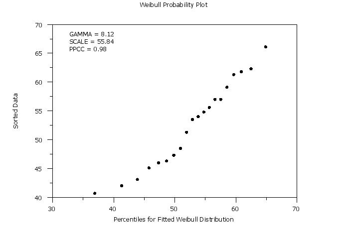
title case asis
label case asis
title Weibull Probability Plot
y1label Sorted Data
x1label Percentiles for Fitted Weibull Distribution
character circle
character hw 1 0.75
character fill on
line blank
.
weibull probability plot y
.
let gamma = round(gamma,2)
move 20 85
text Gamma = ^gamma
let ksscale = round(ksscale,2)
move 20 82
text Scale = ^ksscale
let ppcc = round(ppcc,3)
move 20 79
text PPCC = ^ppcc
    

The following output is generated.

             Two-Parameter Weibull (Minimum) Parameter Estimation:
                               Full Sample Case
  
 Summary Statistics:
 Number of Observations:                              20
 Sample Mean:                                   52.64000
 Sample Standard Deviation:                      7.48517
 Sample Minimum:                                40.70000
 Sample Maximum:                                66.09999
  
 Maximum Likelihood:
 Estimate of Scale:                             55.83881
 Estimate of Shape (Gamma):                      8.11761
 Standard Error of Scale:                        1.61954
 Standard Error of Shape:                        1.41527
 Shape/Scale Covariance:                         0.84710
 Log-likelihood:                          -0.6835433E+02
 AIC:                                      0.1407087E+03
 AICc:                                     0.1414145E+03
 BIC:                                      0.1427001E+03
  
 Maximum Likelihood (Bias Corrected):
 Estimate of Scale:                             55.83881
 Estimate of Shape (Gamma):                      7.55464
 Standard Error of Scale:                        1.61954
 Standard Error of Shape:                        1.22578
 Shape/Scale Covariance:                         0.84710
 Log-likelihood:                          -0.6844503E+02
 AIC:                                      0.1408901E+03
 AICc:                                     0.1415959E+03
 BIC:                                      0.1428815E+03
  
             Confidence Interval for Scale Parameter
  
 ---------------------------------------------------------------------------
                      Normal  Approximation  Likelihood Ratio  Approximation
   Confidence          Lower          Upper             Lower          Upper
  Coefficient          Limit          Limit             Limit          Limit
 ---------------------------------------------------------------------------
        50.00       54.74645       56.93119          54.73232       56.93923
        75.00       53.97578       57.70186          53.92918       57.73490
        90.00       53.17490       58.50274          53.06172       58.60202
        95.00       52.66458       59.01306          52.48611       59.18824
        99.00       51.66716       60.01048          51.29590       60.44785
        99.90       50.50966       61.16798          49.77662       62.19297
 ---------------------------------------------------------------------------
  
  
             Confidence Interval for Shape Parameter
  
 ---------------------------------------------------------------------------
                      Normal  Approximation  Likelihood Ratio  Approximation
   Confidence          Lower          Upper             Lower          Upper
  Coefficient          Limit          Limit             Limit          Limit
 ---------------------------------------------------------------------------
        50.00        7.16302        9.07219           7.19360        9.10074
        75.00        6.48955        9.74566           6.57700        9.83032
        90.00        5.78969       10.44552           5.96703       10.62030
        95.00        5.34372       10.89148           5.59468       11.14076
        99.00        4.47210       11.76310           4.90364       12.19666
        99.90        3.46061       12.77459           4.16282       13.48682
 ---------------------------------------------------------------------------
  
  
             Confidence Intervals for Select Percentiles (alpha = 0.050)
  
 (Based on Normal Approximation)
 ---------------------------------------------------------------------------
                          Point       Standard          Lower          Upper
      Percentile       Estimate          Error          Limit          Limit
 ---------------------------------------------------------------------------
           0.500       29.08095        3.66048       21.90653       36.25536
           1.000       31.68303        3.52762       24.76901       38.59707
           5.000       38.72843        3.01713       32.81494       44.64191
          10.000       42.31954        2.69485       37.03772       47.60134
          20.000       46.41828        2.30418       41.90216       50.93437
          30.000       49.17916        2.04763       45.16586       53.19248
          40.000       51.40420        1.86149       47.75574       55.05266
          50.000       53.37375        1.72632       49.99020       56.75730
          60.000       55.24069        1.63762       52.03099       58.45040
          70.000       57.13040        1.60039       53.99371       60.26711
          80.000       59.21016        1.63240       56.01073       62.40959
          90.000       61.88098        1.79006       58.37254       65.38943
          95.000       63.91991        1.98932       60.02091       67.81892
          97.500       65.58001        2.19282       61.28213       69.87788
          99.000       67.39704        2.44995       62.59519       72.19889
          99.500       68.57125        2.63203       63.41255       73.72996
 ---------------------------------------------------------------------------
  
  
             Anderson-Darling Goodness of Fit Test
                    (Fully Specified Model)
  
 Response Variable: Y
  
 H0: The distribution fits the data
 Ha: The distribution does not fit the data
  
 Distribution: WEIBULL
 Location Parameter:                                0.00000
 Scale Parameter:                                  55.83881
 Shape Parameter 1:                                 8.11761
  
 Summary Statistics:
 Number of Observations:                                 20
 Sample Minimum:                                   40.70000
 Sample Maximum:                                   66.09999
 Sample Mean:                                      52.64000
 Sample SD:                                         7.48517
  
 Anderson-Darling Test Statistic Value:             0.29226
 Number of Monte Carlo Simulations:             10000.00000
 CDF Value:                                         0.05700
 P-Value                                            0.94300
  
  
  
 Percent Points of the Reference Distribution
 -----------------------------------
   Percent Point               Value
 -----------------------------------
             0.0    =          0.000
            50.0    =          0.774
            75.0    =          1.237
            90.0    =          1.927
            95.0    =          2.513
            97.5    =          3.033
            99.0    =          3.758
            99.5    =          4.357
  
 Conclusions (Upper 1-Tailed Test)
 ----------------------------------------------
   Alpha    CDF   Critical Value     Conclusion
 ----------------------------------------------
     10%    90%            1.927      Accept H0
      5%    95%            2.513      Accept H0
    2.5%  97.5%            3.033      Accept H0
      1%    99%            3.758      Accept H0