Extreme Winds Software: Dataplot

Extreme Wind Speeds Software: Dataplot
Introduction	Dataplot is a freely downloadable multi-platform (Unix/Linux, Windows 7/8/10, Mac OS X) program for scientific graphics, statistical analysis, and linear/non-linear modeling. The original version of Dataplot was released by James J. Filliben in 1978 with continual enhancements to the present time. The authors are James J. Filliben and Alan Heckert of the Statistical Engineering Division, Information Technology Laboratory, National Institute of Standards and Technology.
Dataplot Capabilities Relevant to the Analysis of Extreme Winds	Dataplot contains a number of features that are relevant for the analysis of extreme winds. Dataplot provides a number of methods for graphing your data. A few specific graphs of interest for extreme value analysis include: Run sequence plots Histograms Kernel density plots Dataplot supports a library of probability functions. This includes cumulative distribution functions, probability density functions, and percent point functions. The library supports 100+ distributions including the five extreme value distributions (Gumbel, Frechet, Weibull/reverse Weibull, generalized Pareto, and generalized extreme value). Dataplot provides a number of different methods for fitting distributional models. Maximum likelihood Dataplot supports a number of analytical estimation methods for the extreme value distributions. For the Gumbel distribution, moment and maximum likelihood estimates are supported. For the 2-parameter Frechet distribution, maximum likelihood estimates are supported. For the 3-parameter Frechet distribution, l-moment and elemental percentile estimates are supported. For the 2-parameter Weibull distribution, maximum likelihood estimates are supported. For the 3-parameter Weibull distribution, maximum likelihood, moment, modified moment, l-moment, and and elemental percentile estimates are supported. For the generalized Pareto distribution, maximum likelihood, moment, l-moment, and elemental percentile estimates are supported. Note that the moment, l-moment, and maximum likelihood estimates work well for restricted ranges of the shape parameter. One advantage of elemental percentile estimates for the generalized Pareto distribution is that they work well over a much broader range of values for the shape parameter. For the generalized extreme value distribution, l-moment and elemental percentile estimates are supported. In most cases, analytic confidence intervals for distribution parameters and select quantiles will also be generated. When they are not, they can be generated via bootstrapping. The PPCC plot can be used to estimate the shape parameter and a probability plot can be used to estimate the location and scale parameters. Confidence intervals for distribution parameters and select quantiles can be generated via bootstrapping. For the generalized Parero, Dataplot supports the de Haan and CME (Conditional Mean Exceedance) estimation methods. Dataplot provides several methods for assessing the goodness of fit of a distributional model. Anderson-Darling goodness of fit Kolmogorov-Smirnov goodness of fit Chi-square goodness of fit Probability plots Histograms with the fitted PDF overlaid are easily generated in Dataplot. Dataplot provides a few capabilities that are specifically for the analysis of extreme values. Conditional mean exceedance plot Peaks over threshold plot
Further Information	Additional information is available at the Dataplot web site.
	Example
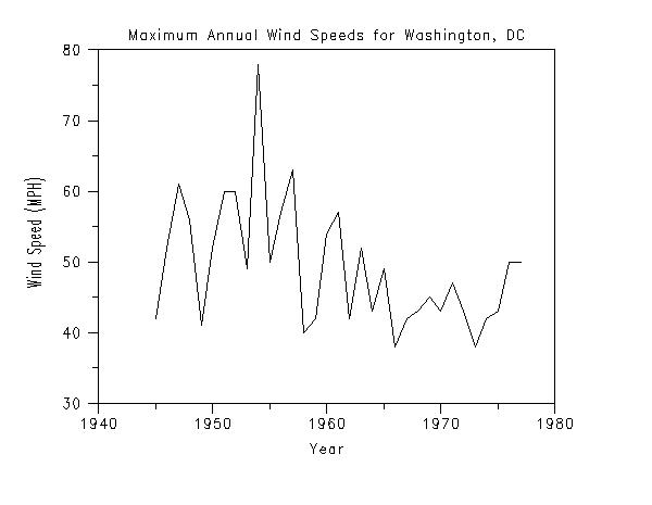
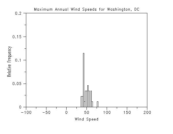
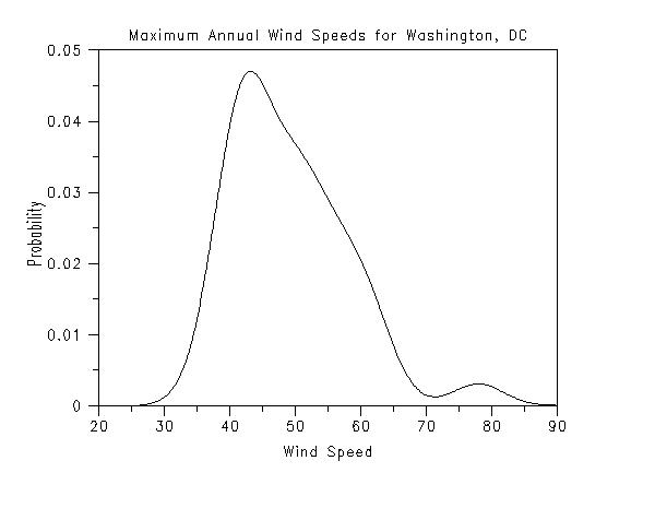
Maximum Annual Wind Speeds for Washington, DC	The following example analyzes a data set containing the maximum annual wind speeds in Washington, DC from 1945 to 1977. The purpose of this example is to illustrate how certain tasks are performed in Dataplot (i.e., it is not meant to be a case study, just a demonstration of some of the basic Dataplot commands used in extreme value analysis). Specifically, the example will demonstrate the following: How to generate preliminary plots of the data How to perform distributional modeling for the extreme value distributions
Read the Data and Generate Preliminary Plots	The first step is to read the data and generate some preliminary plots. This is accomplished with the following Dataplot commands: . . Step 1: Read the Data, define some default . plot control settings . skip 25 read washdc.dat y x title case asis title displacement 2 label case asis . . Step 2: Preliminary Plots of the Data . a. Run Sequence Plot . b. Relative Histogram . c. Kernel Density Plot . title Maximum Annual Wind Speeds for Washington, DC y1label Wind Speed (MPH) x1label Year plot y x . title Maximum Annual Wind Speeds for Washington, DC y1label Relative Frequency x1label Wind Speed relative histogram y . title Maximum Annual Wind Speeds for Washington, DC y1label Probability x1label Wind Speed kernel density plot y The following graphs are generated. We can make the following conclusions based on these plots. 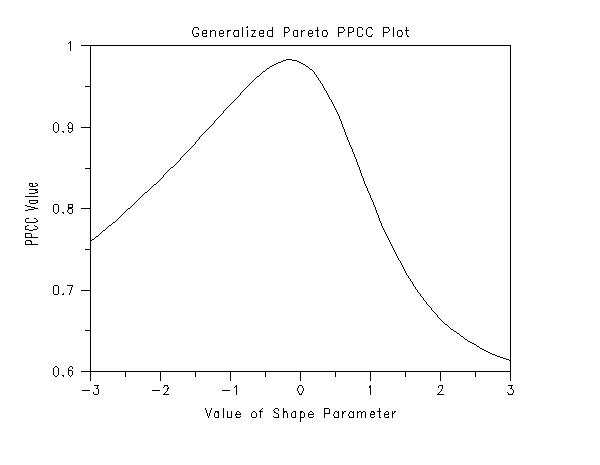The bulk of the annual maximums lie in the range 35 mph to 65 mph. There is one annual maximum that is above 75 mph. The mode of the data is around 45 mph. The data exhibit slight skewing to the right.
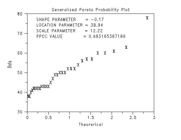
Generalized Pareto Distributional Model	The next step is to develop an appropriate distributional model for the data. A good starting point is to use the generalized Pareto and/or the generalized extreme value distributions since these contain the Gumbel, Frechet, and reverse Weibull as special cases. The following shows the typical steps in developing a generalized Pareto distributional model. We use the PPCC/probability plot approach to estimate the shape, location, and scale parameters. This analysis is performed with the following Dataplot commands. . . Step 3: Generalized Pareto Model . title Generalized Pareto PPCC Plot y1label PPCC Value x1label Value of Shape Parameter generalized pareto ppcc plot y . let gamma = shape title Generalized Pareto Probability Plot x1label Theorerical y1label Data char x line blank generalized pareto probability plot y justification left move 20 85 text Shape Parameter = ^gamma move 20 81 text Location Parameter = ^ppa0 move 20 77 text Scale Parameter = ^ppa1 move 20 73 text PPCC Value = ^maxppcc . let ksloc = ppa0 let ksscale = ppa1 generalized pareto kolm smir goodness of fit y The following graphs and output are generated. KOLMOGOROV-SMIRNOV GOODNESS-OF-FIT TEST NULL HYPOTHESIS H0: DISTRIBUTION FITS THE DATA ALTERNATE HYPOTHESIS HA: DISTRIBUTION DOES NOT FIT THE DATA DISTRIBUTION: GENERALIZED PARETO NUMBER OF OBSERVATIONS = 33 TEST: KOLMOGOROV-SMIRNOV TEST STATISTIC = 0.1334534 ALPHA LEVEL CUTOFF CONCLUSION 10% 0.208 ACCEPT H0 5% 0.231 ACCEPT H0 1% 0.277 ACCEPT H0 We can make the following conclusions based on these plots. The estimate of the shape parameter is -0.18. Note that negative values of the shape parameter indicate that a reverse Weibull is the appropriate model while a value of 0 for the shape parameter indicates that a Gumbel distribution is the appropriate model. Since the estimated shape parameter is negative, but small, the next step will be to fit both a reverse Weibull and a Gumbel model to the data. The probability plot and the Kolmogorov-Smirnov goodness of fit test indicate that the generalized Pareto provides an adequate distributional model.
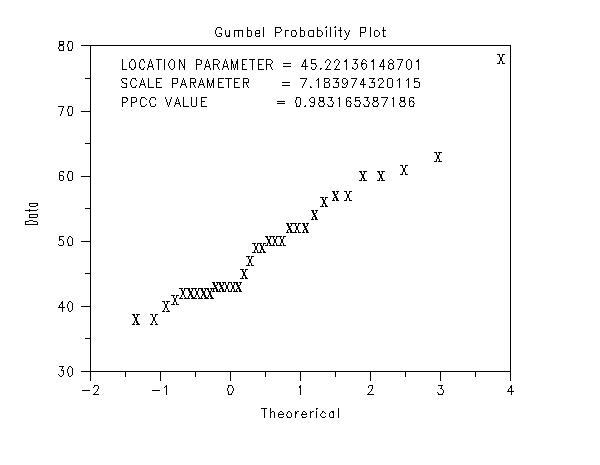
Gumbel Model	The following shows the typical steps in developing a Gumbel distributional model. Perform an Anderson-Darling test to determine if the Gumbel provides an adequate distributional model. Perform a Gumbel maximum likelihood analysis. This analysis provides estimates for the parameters, confidence intervals for the parameters, and estimates and confidence intervals for select percentiles of the distribution. Perform a probability plot analysis. The probability plot provides estimates for location and scale. We then use the bootstrap to provide confidence intervals for the location and scale parameters and for select percentiles. The Anderson-Darling, maximum likelihood estimation, and the probability plot are performed with the following Dataplot commands. . . Step 4: Gumbel Model . set maximum likelihood percentiles default anderson darling gumbel y gumbel mle y . title Gumbel Probability Plot x1label Theorerical y1label Data char x line blank gumbel probability plot y justification left move 20 85 text Location Parameter = ^ppa0 move 20 81 text Scale Parameter = ^ppa1 move 20 77 text PPCC Value = ^maxppcc The following graphs and output are generated. ANDERSON-DARLING 1-SAMPLE TEST THAT THE DATA CAME FROM AN EXTREME VALUE DISTRIBUTION 1. STATISTICS: NUMBER OF OBSERVATIONS = 33 MEAN = 49.21212 STANDARD DEVIATION = 8.813191 LOCATION PARAMETER = 45.35311 SCALE PARAMETER = 6.331326 ANDERSON-DARLING TEST STATISTIC VALUE = 0.6815453 ADJUSTED TEST STATISTIC VALUE = 0.7052736 2. CRITICAL VALUES: 90 % POINT = 0.6370000 95 % POINT = 0.7570000 97.5 % POINT = 0.8770000 99 % POINT = 1.038000 3. CONCLUSION (AT THE 5% LEVEL): THE DATA DO COME FROM AN EXTREME VALUE DISTRIBUTION. GUMBEL MAXIMUM LIKELIHOOD ESTIMATION: FULL SAMPLE, MINIMUM EXTREME VALUES CASE F(X) = (1/s)EXP((X-U)/S)EXP(-EXP((X-U)/S)) U AND S DENOTE THE LOCATION AND SCALE PARAMETERS, RESPECTIVELY STANDARD ERRORS AND CONFIDENCE INTERVALS BASED ON NO BIAS CORRECTION SCALE PARAMETER NUMBER OF OBSERVATIONS = 33 SAMPLE MINIMUM = 38.00000 SAMPLE MAXIMUM = 78.00000 SAMPLE MEAN = 49.21212 SAMPLE STANDARD DEVIATION = 8.813191 MOMENT ESTIMATE OF LOCATION = 53.17859 STANDARD ERROR OF MOMENT ESTIMATE OF LOCATION = 1.292676 MOMENT ESTIMATE OF SCALE = 6.871645 STANDARD ERROR OF MOMENT ESTIMATE OF SCALE = 2.589102 MAXIMUM LIKELIHOOD ESTIMATE OF LOCATION = 53.96301 STANDARD ERROR OF LOCATION ESTIMATE = 1.994741 MAXIMUM LIKELIHOOD ESTIMATE OF SCALE = 10.88288 BIAS CORRECTED ML ESTIMATE OF SCALE = 11.34340 STANDARD ERROR OF SCALE ESTIMATE = 1.477116 STANDARD ERROR OF COVARIANCE = 0.9604377 CONFIDENCE INTERVAL FOR SCALE PARAMETER NORMAL APPROXIMATION CONFIDENCE LOWER UPPER VALUE (%) LIMIT LIMIT ------------------------------------------- 50.000 9.88658 11.8792 75.000 9.18368 12.5821 90.000 8.45324 13.3125 95.000 7.98779 13.7780 99.000 7.07808 14.6877 99.900 6.02241 15.7434 CONFIDENCE INTERVAL FOR LOCATION PARAMETER NORMAL APPROXIMATION CONFIDENCE LOWER UPPER VALUE (%) LIMIT LIMIT ------------------------------------------- 50.000 52.6176 55.3084 75.000 51.6684 56.2577 90.000 50.6820 57.2441 95.000 50.0534 57.8726 99.000 48.8249 59.1011 99.900 47.3993 60.5267 CONFIDENCE LIMITS FOR SELECTED PERCENTILES (BASED ON NORMAL APPROXIMATION): ALPHA = 0.0500 POINT STANDARD LOWER UPPER PERCENTILE ESTIMATE ERROR CONFIDENCE LIMIT CONFIDENCE LIMIT -------------------------------------------------------------------------- 0.5000 35.81701 2.639861 30.64297 40.99104 1.0000 37.34290 2.500051 32.44289 42.24290 5.0000 42.02244 2.140419 37.82729 46.21758 10.0000 44.88634 1.989480 40.98703 48.78565 20.0000 48.78401 1.896091 45.06774 52.50028 30.0000 51.94286 1.926581 48.16683 55.71889 40.0000 54.91441 2.038860 50.91832 58.91050 50.0000 57.95173 2.224468 53.59185 62.31161 60.0000 61.27334 2.490531 56.39199 66.15469 70.0000 65.18251 2.863541 59.57007 70.79495 80.0000 70.28668 3.413945 63.59547 76.97789 90.0000 78.45349 4.379495 69.86983 87.03715 95.0000 86.28729 5.357913 75.78597 96.78861 97.5000 93.97121 6.344194 81.53681 106.4056 99.0000 104.0259 7.657493 89.01752 119.0344 99.5000 111.5967 8.656844 94.62955 128.5638 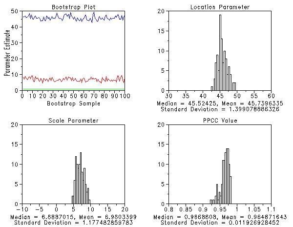The bootstrap analysis is performed with the following Dataplot commands. multiplot 2 2 multiplot corner coordinates 0 0 100 100 multiplot scale factor 1.7 y1label Parameter Estimate x1label x2label Bootstrap Sample title Bootstrap Plot line color blue red green line solid all character blank all set maximum likelihood percentiles default bootstrap gumbel plot y line color black all . skip 0 read dpst1f.dat aloc ascale appcc y1label x2label x3label displacement 16 title Location Parameter let amed = median aloc let amean = mean aloc let asd = sd aloc x2label Median = ^amed, Mean = ^amean x3label Standard Deviation = ^asd histogram aloc title Scale Parameter let amed = median ascale let amean = mean ascale let asd = sd ascale x2label Median = ^amed, Mean = ^amean x3label Standard Deviation = ^asd histogram ascale title PPCC Value let amed = median appcc let amean = mean appcc let asd = sd appcc x2label Median = ^amed, Mean = ^amean x3label Standard Deviation = ^asd histogram appcc x3label displacement . label title . let alpha = 0.05 let xqlow = alpha/2 let xqupp = 1 - alpha/2 . write " " write "Bootstrap-based Confidence Intervals" write "alpha = ^alpha" write " " . let xq = xqlow let loc95low = xq quantile aloc let xq = xqupp let loc95upp = xq quantile aloc let xq = xqlow let sca95low = xq quantile ascale let xq = xqupp let sca95upp = xq quantile ascale write "Confidence Interval for Location: (^loc95low,^loc95upp)" write "Confidence Interval for Scale: (^sca95low,^sca95upp)" serial read p 0.5 1 2.5 5 10 20 30 40 50 60 70 80 90 95 97.5 99 99.5 end of data let nperc = size p skip 1 read matrix dpst4f.dat xqp write " " loop for k = 1 1 nperc let xqptemp = p(k) let amed = median xqp^k let xqpmed(k) = amed let xq = xqlow let atemp = xq quantile xqp^k let xq95low(k) = atemp let xq = xqupp let atemp = xq quantile xqp^k let xq95upp(k) = atemp end of loop set write decimals 3 write "Bootstrap Based Confidence Intervals for Percentiles" variable label p Percentile variable label xqpmed Point Estimate variable label xq95low Lower Confidence Limit variable label xq95upp Upper Confidence Limit write p xqpmed xq95low xq95upp The following graphs and output are generated. Bootstrap-based Confidence Intervals alpha = 0.05 Confidence Interval for Location: (38.04781,47.46314) Confidence Interval for Scale: (5.046363,11.99362) Bootstrap Based Confidence Intervals for Percentiles VARIABLES--P XQPMED XQ95LOW XQ95UPP 0.500 31.574 18.484 36.878 1.000 32.693 20.124 37.621 2.500 34.438 22.720 38.798 5.000 35.985 25.176 39.902 10.000 37.900 28.324 41.326 20.000 40.747 32.631 43.716 30.000 42.765 36.094 46.003 40.000 44.838 39.026 48.151 50.000 46.861 42.295 49.990 60.000 49.119 45.861 52.223 70.000 51.987 48.823 55.697 80.000 55.818 51.981 60.479 90.000 61.794 56.233 68.808 95.000 67.525 59.952 76.792 97.500 73.342 63.533 84.925 99.000 80.621 68.212 95.665 99.500 86.158 71.735 104.009 We can make the following conclusions based on this analysis. The Anderson-Darling test indicates that the Gumbel provides an adequate distributional model for data, although this is somewhat borderline (the Anderson-Darling accepts the Gumbel at the 5% level but rejects at the 10% level). The maximum likelihood and probability plot estimates of location and scale are somewhat different (53.96 and 10.88 compared to 45.22 and 7.18).
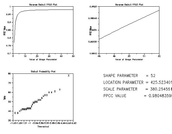
Reverse Weibull Model	The following shows the typical steps in developing a reverse Weibull distributional model. We use the PPCC/probability plot approach to estimate the shape, location, and scale parameters. We could obtain confidence intervals for the parameters and for select quantiles using the bootstrap in a similar manner as we did for the Gumbel distribution. However, we have not included that here. This analysis is performed with the following Dataplot commands. . . Step 5: Reverse Weibull Model . multiplot 2 2 multiplot corner coordinates 0 0 100 100 multiplot scale factor 1 set minmax 2 . set ipl1na rweippcc.jpg device 2 gd jpeg title Reverse Weibull PPCC Plot y1label PPCC Value x1label Value of Shape Parameter weibull ppcc plot y let gamma1 = shape - 2 let gamma2 = shape + 2 if gamma1 <= 0 let gamma1 = 0.1 end of if . weibull ppcc plot y . let gamma = shape title Weibull Probability Plot x1label Theorerical y1label Data char x line blank weibull probability plot y . Generate a null plot so text will go in right spot plot justification left hw 4 2 move 20 85 text Shape Parameter = ^gamma move 20 75 text Location Parameter = ^ppa0 move 20 65 text Scale Parameter = ^ppa1 move 20 55 text PPCC Value = ^maxppcc . end of multiplot device 2 close . let ksloc = ppa0 let ksscale = ppa1 capture wei1.out weibull kolm smir goodness of fit y end of capture The following graphs and output are generated. KOLMOGOROV-SMIRNOV GOODNESS-OF-FIT TEST NULL HYPOTHESIS H0: DISTRIBUTION FITS THE DATA ALTERNATE HYPOTHESIS HA: DISTRIBUTION DOES NOT FIT THE DATA DISTRIBUTION: WEIBULL NUMBER OF OBSERVATIONS = 33 TEST: KOLMOGOROV-SMIRNOV TEST STATISTIC = 0.1682307 ALPHA LEVEL CUTOFF CONCLUSION 10% 0.208 ACCEPT H0 5% 0.231 ACCEPT H0 1% 0.277 ACCEPT H0 We can make the following conclusions based on these plots. The Kolmogorov-Smirnov goodness of fit test indicates the reverse Weibull provides an adequate distributional model. Using the reverse Weibull does not increase the PPCC value (in fact, it actually decreases from 0.983 to 0.980). Based on this, we might be inclined to use the simpler Gumbel model.
[Extreme Winds Home \| SED Home \| Structures Group ] Date created: 03/05/2005 Last updated: 04/26/2023 Please email comments on this WWW page to SED_webmaster@nist.gov

Extreme Wind Speeds Software: Dataplot