
|
|
Extreme Wind Speeds Software: Excel |
|
| Introduction |
In this section, we provide an example of using Excel to
model extreme wind data using a Gumbel distribution.
Note that Excel does not provide some of the sophisticated distributional modeling capabilities that are typically available in statistical programs (e.g., parameter estimation for many different distributions, probability plots for distributions other than the normal, goodness of fit tests, confidence intervals for parameter estimates and quantiles). There are "add-on" programs for Excel that provide more sophisticated statistical capabilities (we do not discuss these other than to mention that they are available). If you have experience writing VBScript macros, you can also implement some of these capabilities by writing your own macros. On the plus side, many engineers and scientists store their data as Excel worksheets, so performing the analysis in Excel can be more convenient. There are relatively simple estimation procedures for the Gumbel distribution that can be implemented in Excel in a straightforward manner, so we will focus on those in this section. If you want to model extreme wind data using a generalized Pareto, reverse Weibull, extreme value type II (Frechet) or generalized extreme value distribution, we recommend you investigate some of the Excel add-on software that provides more advanced statistical capabilities. We also provide links to a number of Excel spreadsheets that perform a similar analysis. |
| Example: Fort Wayne, IN |
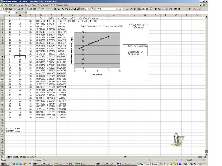
Below is a snapshot of an Excel worksheet containing annual
maximum wind speeds for Fort Wayne, IN for the years 1942-1977.
See below for the source
and background for this data set.
The worksheet contains the following columns:
|
|
|
|
|
|
|
|||||||||||||||||||||||||||||||||||||||||||||||||||||||||||||||||||||||||||||||||||||||||||||||||||||||||||||||||||||||||||||||||||||||||||||||||||||||||||||||||||||||||||||||||||||||||||||||||||||||||||||||||||||||||||||||
| Data for Example in HTML Table |
For clarity, we print the data in the above table as an HTML
table.
|
||||||||||||||||||||||||||||||||||||||||||||||||||||||||||||||||||||||||||||||||||||||||||||||||||||||||||||||||||||||||||||||||||||||||||||||||||||||||||||||||||||||||||||||||||||||||||||||||||||||||||||||||||||||||||||||
|
|
|||||||||||||||||||||||||||||||||||||||||||||||||||||||||||||||||||||||||||||||||||||||||||||||||||||||||||||||||||||||||||||||||||||||||||||||||||||||||||||||||||||||||||||||||||||||||||||||||||||||||||||||||||||||||||||||
| Worksheet Computations | |||||||||||||||||||||||||||||||||||||||||||||||||||||||||||||||||||||||||||||||||||||||||||||||||||||||||||||||||||||||||||||||||||||||||||||||||||||||||||||||||||||||||||||||||||||||||||||||||||||||||||||||||||||||||||||||
| Sort the Data | Once the maximum annual wind speeds were entered into the Excel spreadsheet, they need to be sorted in ascending order from the smallest to the largest. This can be accomplished in Excel by selecting the "Data" button on the toolbar at the top of the page. Then select the "Sort" button in the "Data" menu (this is the first option in the menu). If there is data next to the wind speeds, selecting the "Sort" button results in a "Sort Warning." Select "Continue with Current Selection." After this is selected (or if there is no data next to the wind speed column), the sort menu will appear. Select (if not selected already) Sort by V, select "ascending" and then click the "OK" button. At this point, Excel will properly sort the data. | ||||||||||||||||||||||||||||||||||||||||||||||||||||||||||||||||||||||||||||||||||||||||||||||||||||||||||||||||||||||||||||||||||||||||||||||||||||||||||||||||||||||||||||||||||||||||||||||||||||||||||||||||||||||||||||||
| Creating the Ranks Column | The ranks, or m column can be created by first typing a "1" into the m column next to the first annual maximum wind speed. Next, select "1" and drag the cursor down from the "1" in the new column down the cell in the column that is is directly next to the final annual maxima in the data set. Then select "Edit" in the toolbox at the top of the screen. From the "Edit" menu, select the "Fill" command and once in the Fill menu select "Series." Once in the "Series" box, have the "Series in" columns, of the linear "Type" and with "Step Value" of 1. Set "Stop Value" to the same number as the number of annual maxima in the respective data set (36 in this example). | ||||||||||||||||||||||||||||||||||||||||||||||||||||||||||||||||||||||||||||||||||||||||||||||||||||||||||||||||||||||||||||||||||||||||||||||||||||||||||||||||||||||||||||||||||||||||||||||||||||||||||||||||||||||||||||||
| Creating the N Column | The number of annual maxima, or N column, is created by first typing the number of annual maxima (36 in our example) into the N column next to the m column. Select this number and then go to the "Edit" toolbar and select "Copy." Next, drag the cursor down from the "36" (or whatever the number happens to be for your data set) in the new column down the cell in the column that is directly next to the final number (36 in this example) in the m column. Go to the "Edit" menu a second time and select "Paste." The column is created. | ||||||||||||||||||||||||||||||||||||||||||||||||||||||||||||||||||||||||||||||||||||||||||||||||||||||||||||||||||||||||||||||||||||||||||||||||||||||||||||||||||||||||||||||||||||||||||||||||||||||||||||||||||||||||||||||
| Creating the Pv, -ln(Pv), and -ln(-ln(Pv)) Columns |
The next step in creating this worksheet is to create
equations to solve Pv (the Gringorten estimation of
probability). In Excel, create a new column entitled "Pv".
Select cell "D2" (or the first cell in the column that is
being used). Select the "fx" box above. An equal
sign will appear. From this point, type the equation as
shown in Step 1 except:
N = C2 (or first cell number in N column)
A similar procedure can be followed to create the -ln(Pv) and the -ln(-ln(Pv) columns (note that "ln" is the command for the natural log). |
||||||||||||||||||||||||||||||||||||||||||||||||||||||||||||||||||||||||||||||||||||||||||||||||||||||||||||||||||||||||||||||||||||||||||||||||||||||||||||||||||||||||||||||||||||||||||||||||||||||||||||||||||||||||||||||
| Once the data has been created in the columns, the next step is to graph and fit the data. | |||||||||||||||||||||||||||||||||||||||||||||||||||||||||||||||||||||||||||||||||||||||||||||||||||||||||||||||||||||||||||||||||||||||||||||||||||||||||||||||||||||||||||||||||||||||||||||||||||||||||||||||||||||||||||||||
| Graph the Data | |||||||||||||||||||||||||||||||||||||||||||||||||||||||||||||||||||||||||||||||||||||||||||||||||||||||||||||||||||||||||||||||||||||||||||||||||||||||||||||||||||||||||||||||||||||||||||||||||||||||||||||||||||||||||||||||
| Graph V versus -ln(-ln(Pv)) |
Graph V versus ln(-ln(Pv)). If the data can be
reasonably approximated by a Gumbel distribution, this graph
should be approximately linear. If the graph is not
approximately linear, this indicates that the Gumbel
distribution is not an appropriate distributional model for
the data.
Note that this is essentially a probability plot with V denoting the quantiles of the data and ln(-ln(Pv)) denoting the quantiles of the theoretical Gumbel distribution. The theoretical quantiles are obtained by computing the Gumbel percent point (or inverse cumulative distribution) function on the Pv values. To generate this graph, make sure that no value in any column is selected. Then select the graph icon on the toolbar (blue, yellow, and red bars).
|
||||||||||||||||||||||||||||||||||||||||||||||||||||||||||||||||||||||||||||||||||||||||||||||||||||||||||||||||||||||||||||||||||||||||||||||||||||||||||||||||||||||||||||||||||||||||||||||||||||||||||||||||||||||||||||||
| Fit the Data | |||||||||||||||||||||||||||||||||||||||||||||||||||||||||||||||||||||||||||||||||||||||||||||||||||||||||||||||||||||||||||||||||||||||||||||||||||||||||||||||||||||||||||||||||||||||||||||||||||||||||||||||||||||||||||||||
| Estimates for Location and Scale |
The estimates of the location and scale parameters can be
obtained by fitting a line to the points on the plot.
The slope is an estimate of the scale parameter and the
intercept is an estimate of the location parameter.
In Excel, this fitting can be performed by right clicking on the newly created chart and selecting "Add Trendline." In the "Type" tab, select Linear and under the "Options" tab check to display the equation and the R2 on the chart. Then click "OK." |
||||||||||||||||||||||||||||||||||||||||||||||||||||||||||||||||||||||||||||||||||||||||||||||||||||||||||||||||||||||||||||||||||||||||||||||||||||||||||||||||||||||||||||||||||||||||||||||||||||||||||||||||||||||||||||||
| Values for the Location, Scale and R2 |
The spreadsheet now shows the graph of V versus
ln(-ln(Pv)) along with the equation for the fitted
line. It also shows the R2 value for
the fit. R2 is the square of the
correlation coeffiicent of the points being fit and
provides an indication of how well the data are fit
by this linear fit. A value of 0 indicates no
correlation and a value of 1 indicates perfect positive
correlation.
In the example given here, the intercept (i.e., the estimate of the location parameter) is 50.117 and the slope (i.e., the estimate of the scale parameter) is 5.2058. The R2 value is 0.9627. |
||||||||||||||||||||||||||||||||||||||||||||||||||||||||||||||||||||||||||||||||||||||||||||||||||||||||||||||||||||||||||||||||||||||||||||||||||||||||||||||||||||||||||||||||||||||||||||||||||||||||||||||||||||||||||||||
| Estimate Wind Speeds for a Given Return Period |
Once you have determined that the Gumbel distribution provides
an adequate distributional model and have estimated the
location and scale parameters, you can estimate the extreme
wind speeds for a given return period, R, using the
equation:
with G denoting the percent point (or inverse cumulative distribution) function of the Gumbel distribution. The Gumbel percent point function is
with p denoting the desired quantile. That is, from R we compute a desired quantile. We then apply the percent point function to this quantile to determine the maximum wind speed that corresponds to the desired return interval. For example if you want to know the maximum wind expected in the next 100 years:
-LN(-LN(0.99)) = 74.271. So for this particular example, the 100-year wind is found to be approximately 74 mph. This computation can be performed for any desired return period. The following table shows the computations performed by Excel.
|
||||||||||||||||||||||||||||||||||||||||||||||||||||||||||||||||||||||||||||||||||||||||||||||||||||||||||||||||||||||||||||||||||||||||||||||||||||||||||||||||||||||||||||||||||||||||||||||||||||||||||||||||||||||||||||||
| Excel Spreadsheets | |||||||||||||||||||||||||||||||||||||||||||||||||||||||||||||||||||||||||||||||||||||||||||||||||||||||||||||||||||||||||||||||||||||||||||||||||||||||||||||||||||||||||||||||||||||||||||||||||||||||||||||||||||||||||||||||
| NBS Building Science Seris 118 |
The data for the above example is from Simiu, Changery, and
Filliben (1979), "Extreme Wind Speeds at 129 Stations in the
Contiguous United States," NBS Building Science Series 118.
Note that in this publication the values for return periods are different from those that have been calculated in these examples. The differences are typically of the order of 1-2% and are due to the different estimation methods being used. Means and standard deviations have also been calculated for the rounded off values and are located in the Excel spreadsheet. |
||||||||||||||||||||||||||||||||||||||||||||||||||||||||||||||||||||||||||||||||||||||||||||||||||||||||||||||||||||||||||||||||||||||||||||||||||||||||||||||||||||||||||||||||||||||||||||||||||||||||||||||||||||||||||||||
| Links to Excel Spreadsheets |
The following links are to Excel spreadsheets derived from
NBS 118 that contain the data and extreme value type I (Gumbel)
estimation for 129 stations across the United States. In
hurricane zones, the estimation methods may have to be
different from those used for non-hurricane regions (see
Simiu and Scanlan,
Chapter 3). Some of the locations shown have the
indication "Caution - Hurricane Zone" on the graph.
All of the wind speeds used in this analysis have been corrected to represent fastest-mile wind speed at 10 meters above ground level. The ratio of 50-year peak gust to 50-year fastest mile gusts is roughly 1.20.
|
||||||||||||||||||||||||||||||||||||||||||||||||||||||||||||||||||||||||||||||||||||||||||||||||||||||||||||||||||||||||||||||||||||||||||||||||||||||||||||||||||||||||||||||||||||||||||||||||||||||||||||||||||||||||||||||
|
|
|||||||||||||||||||||||||||||||||||||||||||||||||||||||||||||||||||||||||||||||||||||||||||||||||||||||||||||||||||||||||||||||||||||||||||||||||||||||||||||||||||||||||||||||||||||||||||||||||||||||||||||||||||||||||||||||
|
Date created: 05/06/2005 |
|||||||||||||||||||||||||||||||||||||||||||||||||||||||||||||||||||||||||||||||||||||||||||||||||||||||||||||||||||||||||||||||||||||||||||||||||||||||||||||||||||||||||||||||||||||||||||||||||||||||||||||||||||||||||||||||